3 + 5[1] 812 / 7[1] 1.714286By the end of this class, you should
The term “R” is used to refer to both the programming language and the software that interprets the scripts written using it.
RStudio is a popular way to write R scripts and interact with the R software. To function correctly, RStudio needs R and therefore both need to be installed on your computer.
In R, the results of your analysis rely on a series of written commands, and not on remembering a succession of pointing and clicking. That is a good thing! So, if you want to redo your analysis because you collected more data, you don’t have to remember which button you clicked in which order to obtain your results. With a stored series of commands in an R script, you can repeat running them and R will process the new dataset exactly the same way as before.
Working with scripts makes the steps you used in your analysis clear, and the code you write can be inspected by someone else who can give you feedback and spot mistakes.
Working with scripts forces you to have a deeper understanding of what you are doing, and facilitates your learning and comprehension of the methods you use.
Reproducibility is when someone else, including your future self, can obtain the same results from the same dataset when using the same analysis.
R integrates with other tools to generate manuscripts from your code. If you collect more data, or fix a mistake in your dataset, the figures and the statistical tests in your manuscript are updated automatically.
R is widely used in academia and in industries such as pharma and biotech. These organisations expect analyses to be reproducible, so knowing R will give you an edge with these requirements.
With 10,000+ packages that can be installed to extend its capabilities, R provides a framework that allows you to combine statistical approaches from many scientific disciplines to best suit the analytical framework you need to analyze your data. For instance, R has packages for image analysis, GIS, time series, population genetics, and a lot more.
The skills you learn with R scale easily with the size of your dataset. Whether your dataset has hundreds or millions of lines, it won’t make much difference to you.
R is designed for data analysis. It comes with special data structures and data types that make handling of missing data and statistical factors convenient.
R can connect to spreadsheets, databases, and many other data formats, on your computer or on the web.
The plotting functionalities in R are endless, and allow you to adjust any aspect of your graph to visualize your data more effectively.
Thousands of people use R daily. Many of them are willing to help you through mailing lists and websites such as Stack Overflow, RStudio community, and Slack channels such as
the R for Data Science online community (https://www.rfordatasci.com/). In addition, there are numerous online and in person meetups organised globally through organisations such as R Ladies Global (https://rladies.org/).
Anyone can inspect the source code to see how R works. Because of this transparency, there is less chance for mistakes, and if you (or someone else) find some, you can report and fix bugs.
Let’s start by learning about RStudio, which is an Integrated Development Environment (IDE) for working with R.
The RStudio IDE open-source product is free under the Affero General Public License (AGPL) v3. The RStudio IDE is also available with a commercial license and priority email support from RStudio, PBC.
We will use RStudio IDE to write code, navigate the files on our computer, inspect the variables we are going to create, and visualize the plots we will generate. RStudio can also be used for other things (e.g., version control, developing packages, writing Shiny apps) that we will not cover during the workshop.
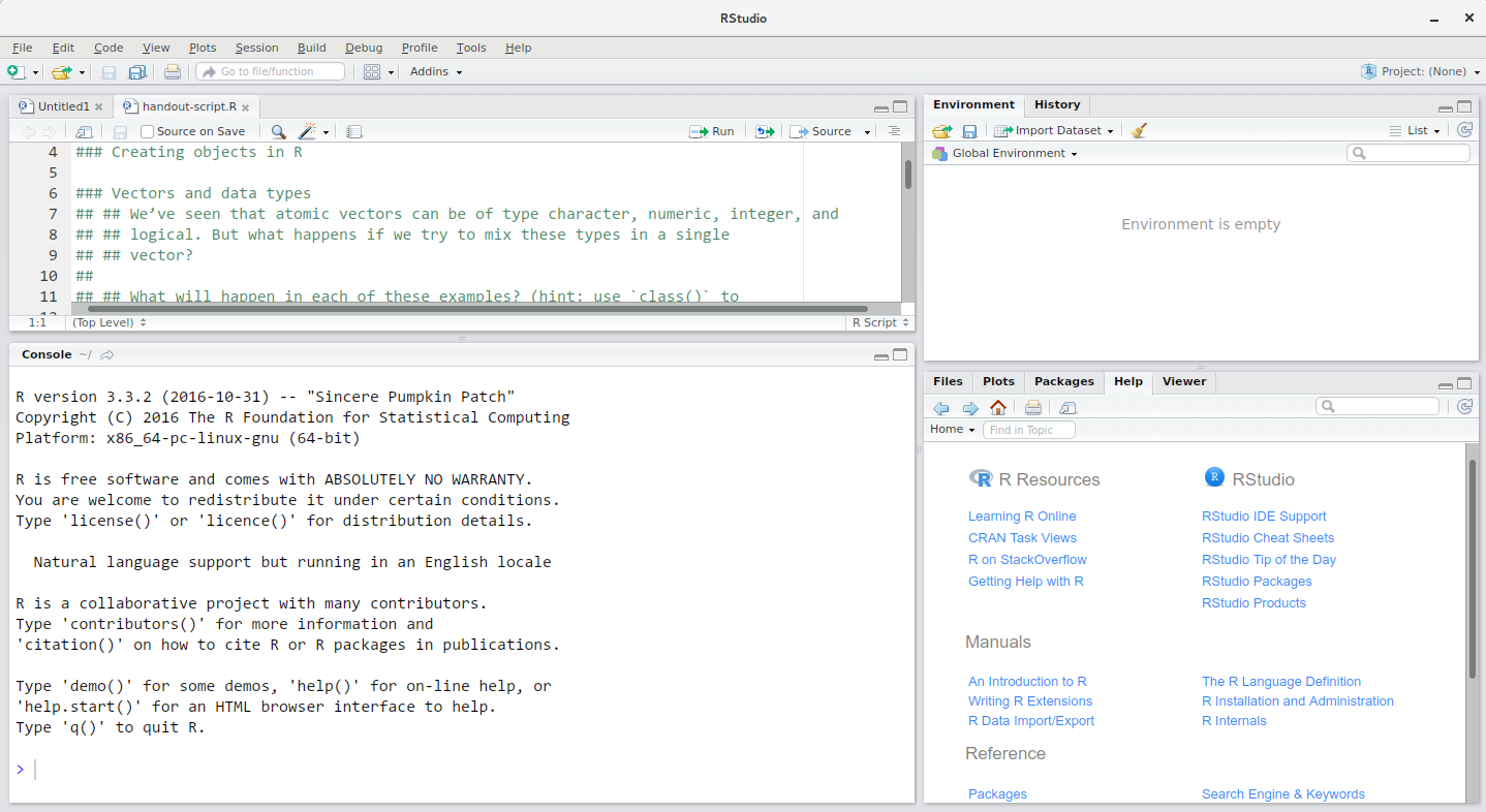
RStudio is divided into 4 “panes”:
The placement of these panes and their content can be customized (see menu, Tools -> Global Options -> Pane Layout). For ease of use, settings such as background color, font color, font size, and zoom level can also be adjusted in this menu (Global Options -> Appearance).
One of the advantages of using RStudio is that all the information you need to write code is available in a single window. Additionally, with many shortcuts, autocompletion, and highlighting for the major file types you use while developing in R, RStudio will make typing easier and less error-prone.
It is good practice to keep a set of related data, analyses, and text self-contained in a single folder, called the working directory. All of the scripts within this folder can then use relative paths to files that indicate where inside the project a file is located (as opposed to absolute paths, which point to where a file is on a specific computer). Working this way allows you to move your project around on your computer and share it with others without worrying about whether or not the underlying scripts will still work.
RStudio provides a helpful set of tools to do this through its “Projects” interface, which not only creates a working directory for you, but also remembers its location (allowing you to quickly navigate to it) and optionally preserves custom settings and (re-)open files to assist resume work after a break. Go through the steps for creating an “R Project” for this tutorial below.
File menu, click on New Project. Choose New Directory, then New Project.Create Project (check the box that says “Create a git repository”).Let’s review what happened: we created a new R project, and RStudio opened the project.
Look at the file pane in the lower-right. You should see some files that were newly created by RStudio: .gitgnore and day03-practice.Rproj.
We learned about .gitignore last week. By default, RStudio creates a .gitignore file for you that lists files that your project should ignore; you can open it to see what is says if you want, but leave it as it is.
The .Rproj file contains settings used by RStudio for your project. Generally, you don’t edit it by hand. But it does have one other very useful function: when you want to start working on a project, you can double-click that file, and RStudio will open with the project loaded. Let’s try this. I think this is the easiest way to re-open a project.
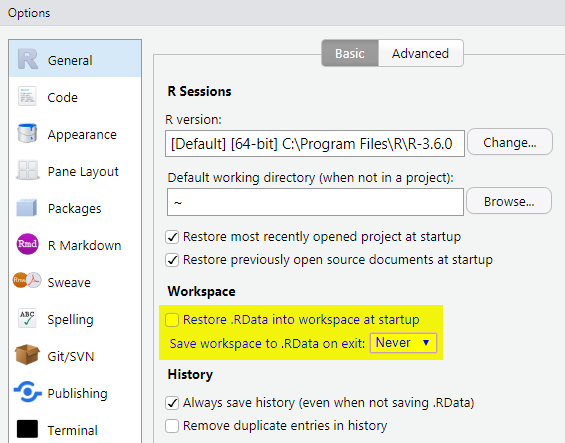
Click “Tools” -> “Global Options”, then under “Workspace” de-select “Restore .RData into workspace at startup” and set “Save workspace to .RData on exit” to “Never”.
A workspace is your current working environment in R which includes any user-defined object. By default, all of these objects will be saved, and automatically loaded, when you reopen your project. Saving a workspace to .RData can be cumbersome, especially if you are working with larger datasets, and it can lead to hard to debug errors by having objects in memory you forgot you had. Therefore, it is often a good idea to turn this off.
You can get output from R simply by typing math in the console:
3 + 5[1] 812 / 7[1] 1.714286However, to do useful and interesting things, we need to assign values to objects. To create an object, we need to give it a name followed by the assignment operator <-, and the value we want to give it:
weight_kg <- 55<- is the assignment operator. It assigns values on the right to the object on the left. So, after executing x <- 3, the value of x is 3. For historical reasons, you can also use = for assignments, but not in every context. Because of the slight differences in syntax, it is good practice to always use <- for assignments.
In RStudio, typing Alt + - (push Alt at the same time as the - key) will write <- in a single keystroke in a PC, while typing Option + - (push Option at the same time as the - key) does the same in a Mac.
Objects can be given almost any name such as x, current_temperature, or subject_id. Here are some further guidelines on naming objects:
2x is not valid, but x2 is).weight_kg is different from Weight_kg.if, else, for, see here for a complete list). In general, even if it’s allowed, it’s best to not use other function names (e.g., c, T, mean, data, df, weights). If in doubt, check the help to see if the name is already in use..) within names. Many function names in R itself have them and dots also have a special meaning (methods) in R and other programming languages. To avoid confusion, don’t include dots in names.lintr package to automatically check for issues in the styling of your code.What are known as objects in R are known as variables in many other programming languages. Depending on the context, object and variable can have drastically different meanings. However, in this lesson, the two words are used synonymously. For more information see: https://cran.r-project.org/doc/manuals/r-release/R-lang.html#Objects
When assigning a value to an object, R does not print anything. You can force R to print the value by using parentheses or by typing the object name:
weight_kg <- 55 # doesn't print anything
(weight_kg <- 55) # but putting parenthesis around the call prints the value of `weight_kg`
[1] 55weight_kg # and so does typing the name of the object[1] 55Now that R has weight_kg in memory, we can do arithmetic with it. For instance, we may want to convert this weight into pounds (weight in pounds is 2.2 times the weight in kg):
2.2 * weight_kg[1] 121We can also change an object’s value by assigning it a new one:
weight_kg <- 57.5
2.2 * weight_kg
[1] 126.5This means that assigning a value to one object does not change the values of other objects. For example, let’s store the animal’s weight in pounds in a new object, weight_lb:
weight_lb <- 2.2 * weight_kgand then change weight_kg to 100.
weight_kg <- 100What do you think is the current content of the object weight_lb? 126.5 or 220?
Up to now, your code has been in the console. This is useful for quick queries but not so helpful if you want to revisit your work for any reason. A script can be opened by pressing Ctrl + Shift + N. It is wise to save your script file immediately. To do this press Ctrl + S. This will open a dialogue box where you can decide where to save your script file, and what to name it. The .R file extension is added automatically and ensures your file will open with RStudio.
Don’t forget to save your work periodically by pressing Ctrl + S.
Functions are “canned scripts” that automate more complicated sets of commands including operations assignments, etc. Many functions are predefined, or can be made available by importing R packages (more on that later). A function usually takes one or more inputs called arguments. Functions often (but not always) return a value. A typical example would be the function sqrt(). The input (the argument) must be a number, and the return value (in fact, the output) is the square root of that number. Executing a function (‘running it’) is called calling the function. An example of a function call is:
weight_kg <- sqrt(10)Here, the value of 10 is given to the sqrt() function, the sqrt() function calculates the square root, and returns the value which is then assigned to the object weight_kg. This function takes one argument, other functions might take several.
The return ‘value’ of a function need not be numerical (like that of sqrt()), and it also does not need to be a single item: it can be a set of things, or even a dataset. We’ll see that when we read data files into R.
Arguments can be anything, not only numbers or filenames, but also other objects. Exactly what each argument means differs per function, and must be looked up in the documentation (see below). Some functions take arguments which may either be specified by the user, or, if left out, take on a default value: these are called options. Options are typically used to alter the way the function operates, such as whether it ignores ‘bad values’, or what symbol to use in a plot. However, if you want something specific, you can specify a value of your choice which will be used instead of the default.
Let’s try a function that can take multiple arguments: round().
round(3.14159)[1] 3Here, we’ve called round() with just one argument, 3.14159, and it has returned the value 3. That’s because the default is to round to the nearest whole number. If we want more digits we can see how to do that by getting information about the round function. We can use args(round) to find what arguments it takes, or look at the help for this function using ?round.
args(round)function (x, digits = 0, ...)
NULL?roundWe see that if we want a different number of digits, we can type digits = 2 or however many we want.
round(3.14159, digits = 2)[1] 3.14A vector is the most common and basic data type in R, and is pretty much the workhorse of R. A vector is composed by a series of values, which can be either numbers or characters. We can assign a series of values to a vector using the c() function. For example we can create a vector of animal weights and assign it to a new object weight_g:
weight_g <- c(50, 60, 65, 82)
weight_g
[1] 50 60 65 82A vector can also contain characters:
animals <- c("mouse", "rat", "dog")
animals
[1] "mouse" "rat" "dog" The quotes around “mouse”, “rat”, etc. are essential here. Without the quotes R will assume objects have been created called mouse, rat and dog. As these objects don’t exist in R’s memory, there will be an error message.
There are many functions that allow you to inspect the content of a vector. length() tells you how many elements are in a particular vector:
length(weight_g)[1] 4length(animals)[1] 3An important feature of a vector, is that all of the elements are the same type of data. The function typeof() indicates what kind of object you are working with (notice that R confusingly calls numeric data “double”):
typeof(weight_g)[1] "double"typeof(animals)[1] "character"The function str() provides an overview of the structure of an object and its elements. It is a useful function when working with large and complex objects:
str(weight_g) num [1:4] 50 60 65 82str(animals) chr [1:3] "mouse" "rat" "dog"You can use the c() function to add other elements to your vector:
weight_g <- c(weight_g, 90) # add to the end of the vector
weight_g <- c(30, weight_g) # add to the beginning of the vector
weight_g
[1] 30 50 60 65 82 90In the first line, we take the original vector weight_g, add the value 90 to the end of it, and save the result back into weight_g. Then we add the value 30 to the beginning, again saving the result back into weight_g.
We can do this over and over again to grow a vector, or assemble a dataset. As we program, this may be useful to add results that we are collecting or calculating.
An atomic vector is the simplest R data type and is a linear vector of a single type. Above, we saw 2 of the 6 main atomic vector types that R uses: "character" and "numeric" (or "double"). These are the basic building blocks that all R objects are built from. The other 4 atomic vector types are:
"logical" for TRUE and FALSE (the boolean data type)"integer" for integer numbers (e.g., 2L, the L indicates to R that it’s an integer)"complex" to represent complex numbers with real and imaginary parts (e.g., 1 + 4i) and that’s all we’re going to say about them"raw" for bitstreams that we won’t discuss furtherYou can check the type of your vector using the typeof() function and inputting your vector as the argument.
Vectors are one of the many data structures that R uses. Other important ones are lists (list), matrices (matrix), data frames (data.frame), factors (factor) and arrays (array).
If we want to extract one or several values from a vector, we must provide one or several indices in square brackets. For instance:
animals <- c("mouse", "rat", "dog", "cat")
animals[2]
[1] "rat"animals[c(3, 2)][1] "dog" "rat"We can also repeat the indices to create an object with more elements than the original one:
more_animals <- animals[c(1, 2, 3, 2, 1, 4)]
more_animals
[1] "mouse" "rat" "dog" "rat" "mouse" "cat" R indices start at 1. Programming languages like Fortran, MATLAB, Julia, and R start counting at 1, because that’s what human beings typically do. Languages in the C family (including C++, Java, Perl, and Python) count from 0 because that’s simpler for computers to do.
Another common way of subsetting is by using a logical vector. TRUE will select the element with the same index, while FALSE will not:
weight_g <- c(21, 34, 39, 54, 55)
weight_g[c(TRUE, FALSE, FALSE, TRUE, TRUE)]
[1] 21 54 55Typically, these logical vectors are not typed by hand, but are the output of other functions or logical tests. For instance, if you wanted to select only the values above 50:
weight_g > 50 # will return logicals with TRUE for the indices that meet the condition[1] FALSE FALSE FALSE TRUE TRUE## so we can use this to select only the values above 50
weight_g[weight_g > 50][1] 54 55You can combine multiple tests using & (both conditions are true, AND) or | (at least one of the conditions is true, OR):
weight_g[weight_g > 30 & weight_g < 50][1] 34 39weight_g[weight_g <= 30 | weight_g == 55][1] 21 55weight_g[weight_g >= 30 & weight_g == 21]numeric(0)Here, > for “greater than”, < stands for “less than”, <= for “less than or equal to”, and == for “equal to”. The double equal sign == is a test for numerical equality between the left and right hand sides, and should not be confused with the single = sign, which performs variable assignment (similar to <-).
A common task is to search for certain strings in a vector. One could use the “or” operator | to test for equality to multiple values, but this can quickly become tedious. The function %in% allows you to test if any of the elements of a search vector are found:
animals <- c("mouse", "rat", "dog", "cat", "cat")

# return both rat and cat
animals[animals == "cat" | animals == "rat"]
[1] "rat" "cat" "cat"# return a logical vector that is TRUE for the elements within animals
# that are found in the character vector and FALSE for those that are not
animals %in% c("rat", "cat", "dog", "duck", "goat", "bird", "fish")[1] FALSE TRUE TRUE TRUE TRUE# use the logical vector created by %in% to return elements from animals
# that are found in the character vector
animals[animals %in% c("rat", "cat", "dog", "duck", "goat", "bird", "fish")][1] "rat" "dog" "cat" "cat"Go to Moodle, click on the Day 3 Homework assignment, and click on the link to accept the assignment. This will create the repo in your GitHub account.
Next, clone the remote repo to your local machine. Then, edit the file day_03_homework.R file in RStudio. Make sure that your code runs without errors. Once you have done so, commit your changes and push to the remote. Don’t forget to push! If you don’t push, your work will not be submitted.
You can double check that you’ve successfully submitted (pushed) the homework by visiting your GitHub repo in your browser (use the same link in Moodle that you clicked to accept the assignment). Make sure the homework file there shows the same changes that you made in RStudio.
Be sure to do this BY THE DEADLINE, or your work will not be counted.
These materials were modified by Joel H. Nitta from the Data Carpentry “Data Analysis and Visualization in R for Ecologists” lesson (https://datacarpentry.org/R-ecology-lesson) under the CC BY Attribution 4.0 International license.
Comments
The comment character in R is
#. Anything to the right of a#in a script will be ignored by R. It is useful to leave notes and explanations in your scripts. For convenience, RStudio provides a keyboard shortcut to comment or uncomment a paragraph: after selecting the lines you want to comment, press at the same time on your keyboard Ctrl + Shift + C. If you only want to comment out one line, you can put the cursor at any location of that line (i.e. no need to select the whole line), then press Ctrl + Shift + C.