[1] 4Day 3: Basic usage of R and RStudio
Why use a programming language?
- Programming makes your analysis reproducible, because you have an exact, written record of what you have done
What is reproducibility?
- The ability for other people (including your future self!) to reproduce your analysis results
- Gives you confidence in your results
- Makes it easier to switch between projects
Why learn R?
- R is free
- R is extensible
- R produces high-quality graphics
- R has a large and welcoming community
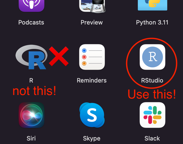
R vs. RStudio
R is the programming language
RStudio is software to use R and write R code
We will always use R through RStudio! (don’t click on the icon for R)
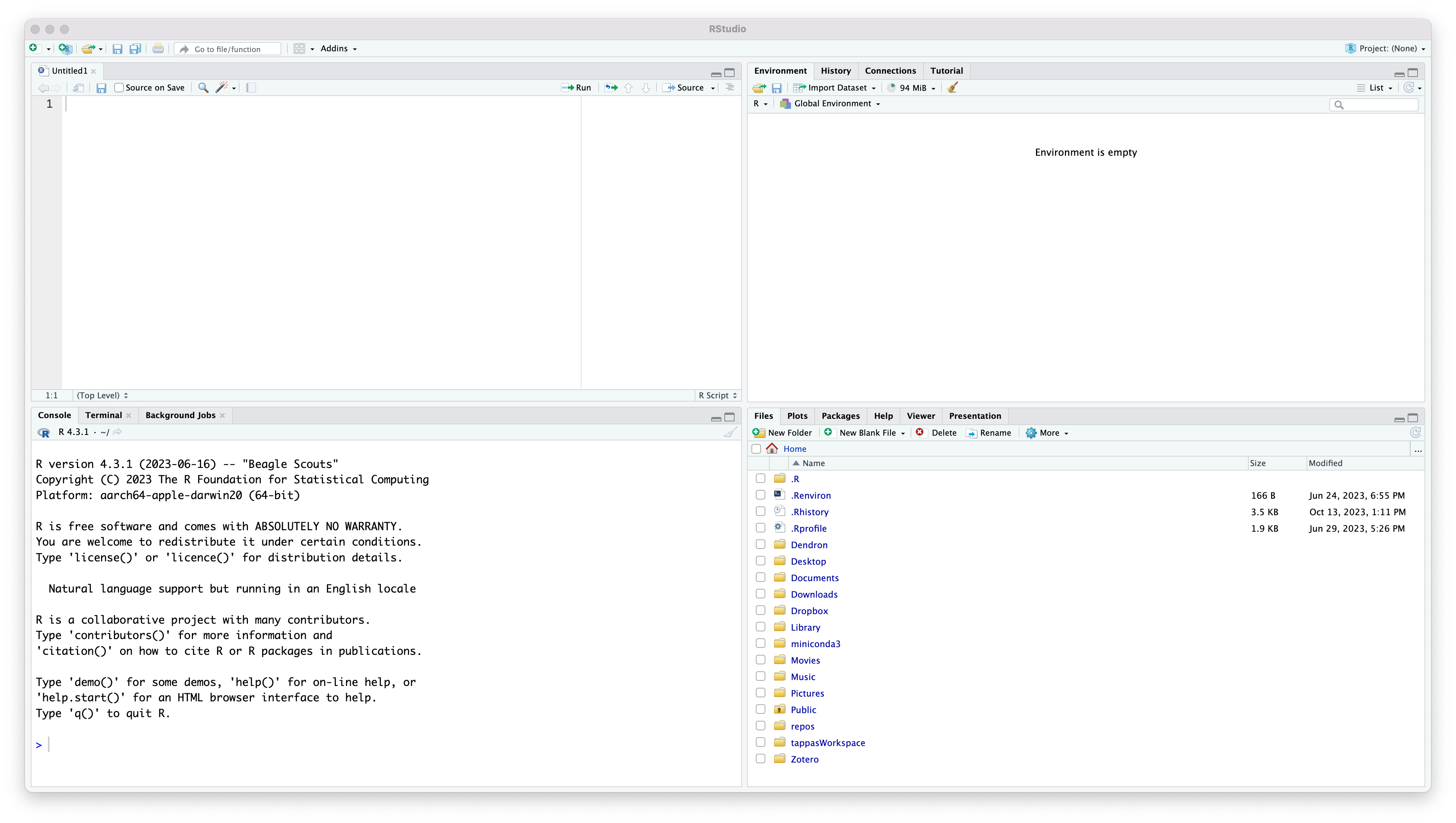
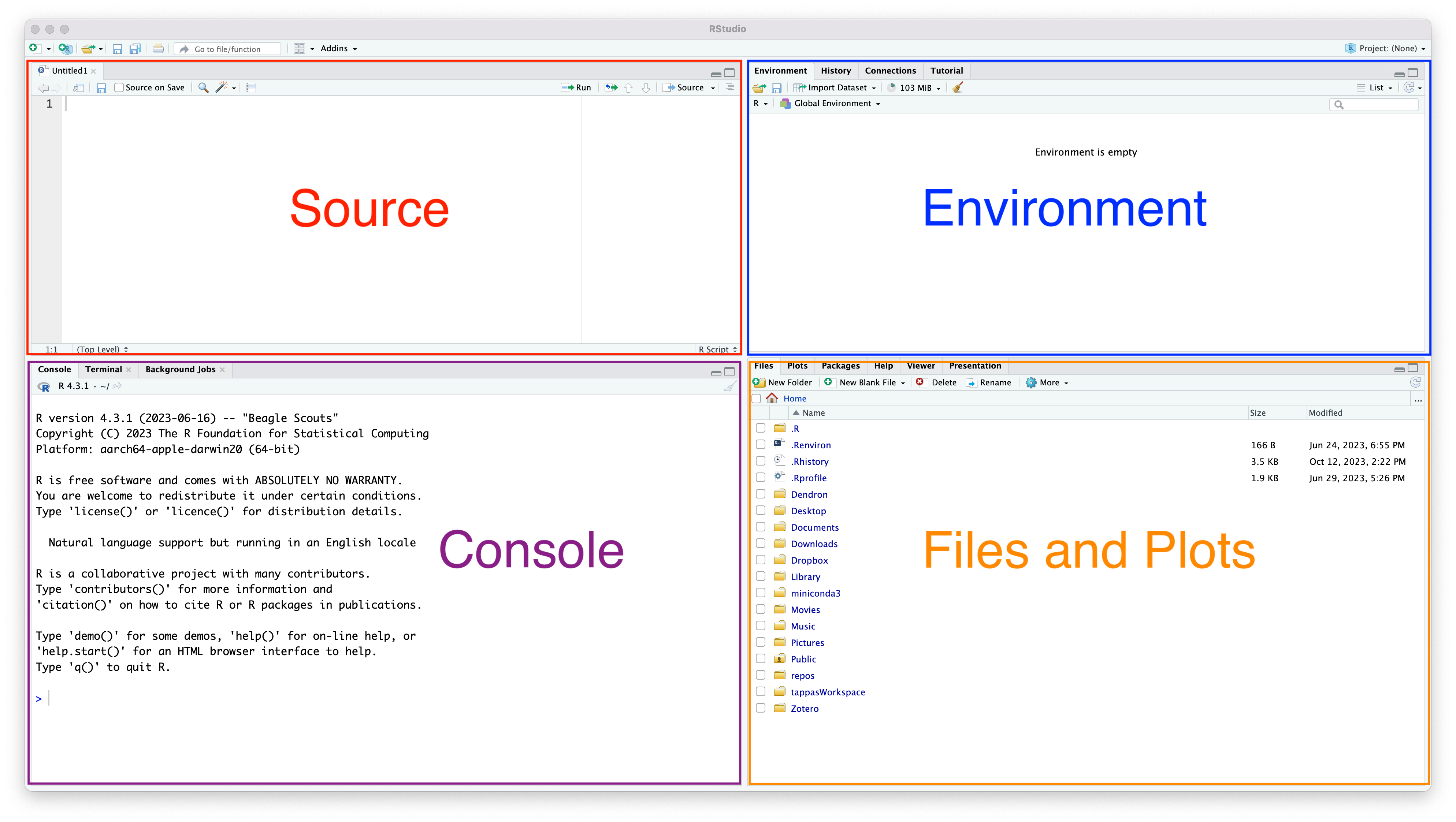
Introduction to RStudio
We will start by navigating RStudio
There are four main panels
- Source (where you write your code)
- Environment (lists the objects in your R session)
- R Console (where you talk to R)
- Files and Plots (shows the files in your project, and any plots you make)
Projects
- An R Project is a folder that contains all the files you need for a particular data analysis project
- Basically the same thing as a repo (if you are using git)
- Projects help organize code and files so we don’t get lost
Create a new project
So far, we have only cloned projects from GitHub
Today you will create a new project on your computer
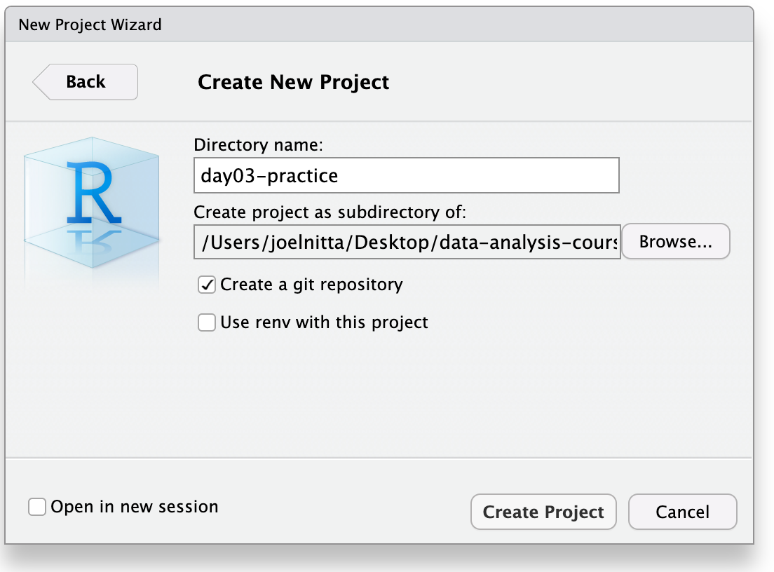
Create a new project
In RStudio, click
File➡︎New Project➡︎New Directory➡︎New Project(again)- Enter the name of the project (folder) and where to put it
- I recommend putting it somewhere easy to find
Let’s put call this project
day03-practiceand put it in thedata-analysis-coursefolder on the DesktopClick “Create a git repository”, since we are using git
Create a new project
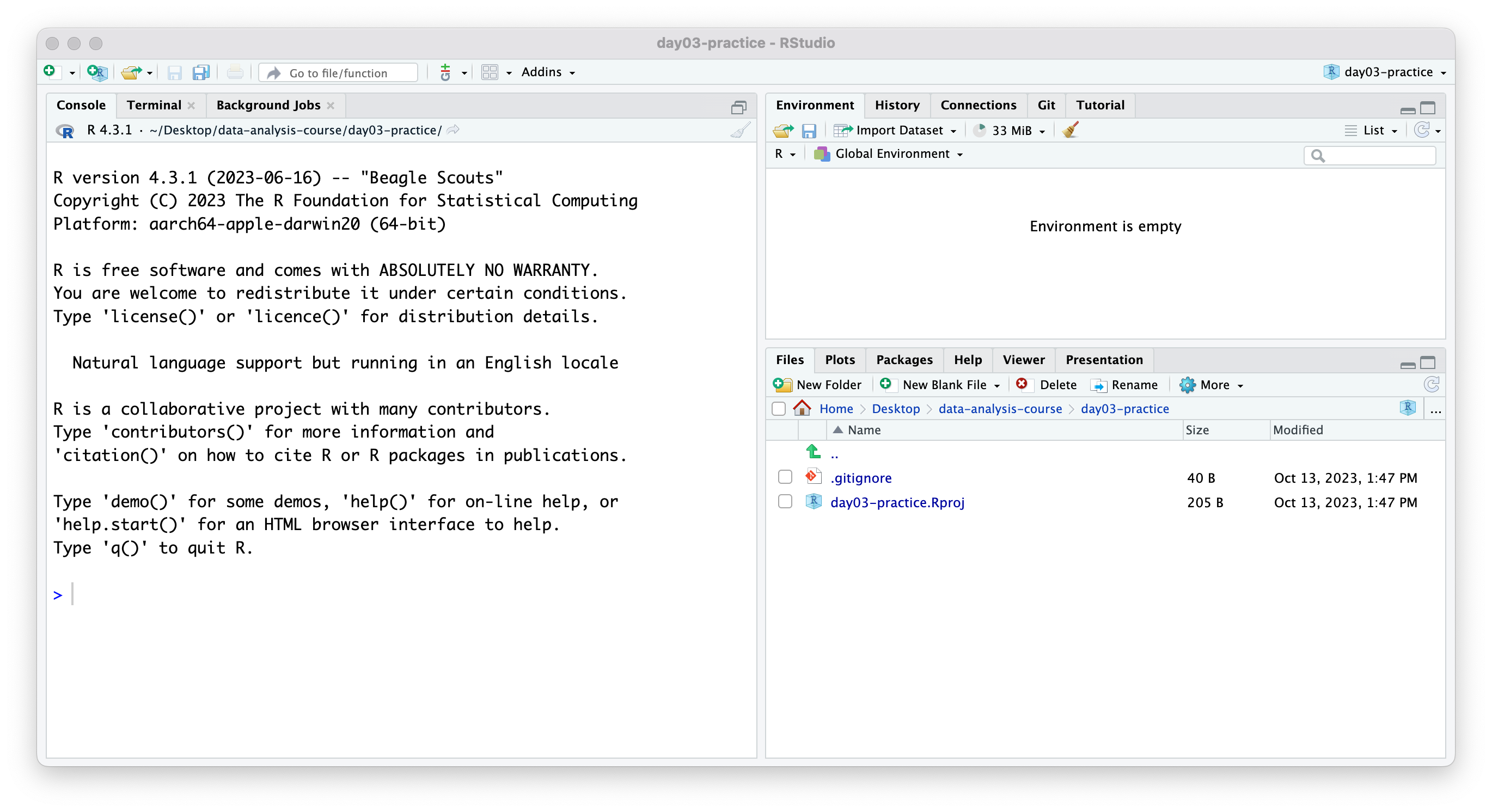
RStudio will restart, and you will see in the File pane that we are located in the new project
RStudio has created two files automatically,
day03-practice.Rprojand.gitignore- Commit these files with the commit message “Initial commit” (or whatever you want, but that is often used as a first commit message for a new project)
Now we are ready to start using R!
R as a calculator
You can execute R code to calculate numbers directly in the console by typing the calculation then pressing “Enter”
Try something like this:
R as a calculator
Congratulations! You are now an R programmer!
Objects (variables)
R can do much more than act like a calculator
One very useful thing is the ability to store values in variables, often called “objects” in R
We assign values to objects using the arrow symbol:
<-
However, R does not show you the value of x when you assign it
Objects (variables)
To check the value of x, type x in the console and press “Enter”
The value of x is also shown in the Environment panel (top-right panel)
Objects (variables)
Now that we have saved a value to x, we can do additional calculations with it:
Objects (variables)
We can then use that code to build a new object:
Objects (variables)
But notice that the objects don’t “react” to each other (in other words, assigning a value to one object does not change the values of other objects):
Workspace settings and using the .Rproj file
Before continuing, we need to change some of the default settings in R
I’ll also demonstrate how to use the
.Rprojfile to open a projectQuit RStudio (we will open it again soon) by clicking
File➡︎Quit Session
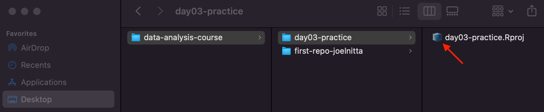
Use the .Rproj file to open the project
- Open your project by navigating to
data-analysis-course/day03-practiceon your Desktop and clicking onday03-practice.Rproj.
Change Workspace settings
- What do you see in RStudio when you open your project?
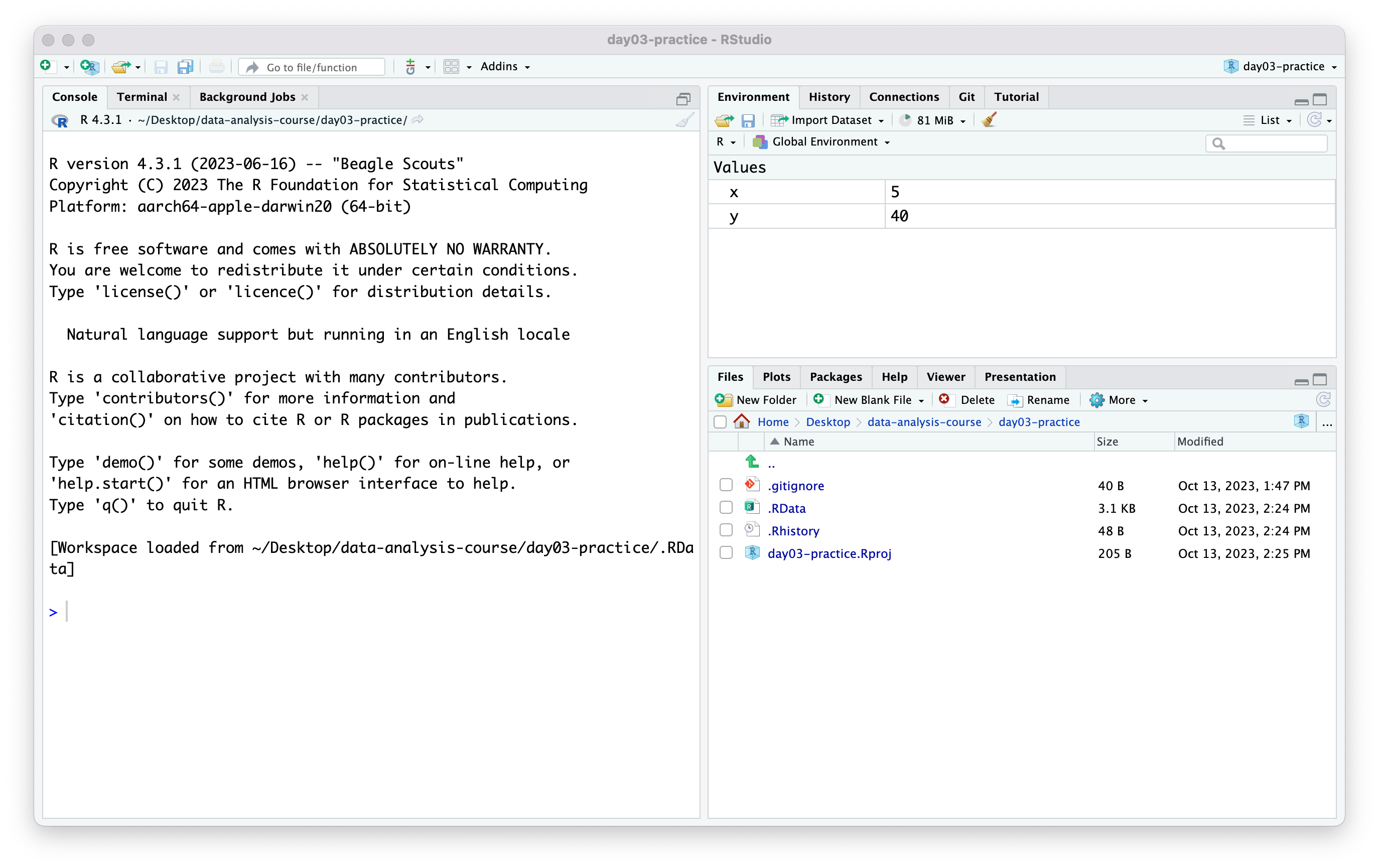
Change Workspace settings
- Notice in the “Environment” pane (upper-right) that
xandyare still there, even though the code that we typed last time is gone!- In other words, we don’t know how we got
xandy - This is bad for reproducibility!
- In other words, we don’t know how we got
Change Workspace settings
- The contents of the R session (the “environment”) should only show what we have done using code during that session
- We will change the default settings to avoid this behavior
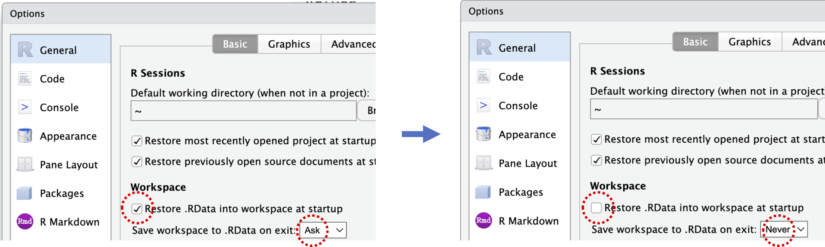
Change Workspace settings
- Click on
Tools➡︎Global Options- Uncheck “Restore .RData into workspace at startup”
- Select “Never” for “Save workspace to .RData on exit”
- Click “OK”
- You can also delete the
.RDatafile, which is where those data were stored
Saving code
- So far, we have only typed code directly into R
- It is much more useful to save your code in a file (called a “script”) so that you can run it again without typing everything all over again
Saving code
Click
File➡︎New File➡︎R ScriptClick the disk icon or
File➡︎Save As...to give your file a name (let’s say, “practice.R”) and save it.
Running code from a file
- Type the same code as before in your new file:
x <- 2 + 2and hit the “Enter” key
Notice that R does not run the code, since this is the file editing pane, not the R console
We need to send the code to the console (that is, send it to R)
Running code from a file
One way to do this is to copy-and-paste it. But that is annoying.
The better way is to use the keyboard shortcut: control (Window) or command (Mac) + the enter key. Try it!
You can also either press the “Run” button in RStudio to run one line at a time, or the “Source” button to run all of the contents of your script
Comments
Functions and arguments
The next step in our R journey is to learn about functions
A function takes input, does something to it, and returns output
For example, let’s try using the
roundfunction, which rounds numbers
Functions and arguments
- The input to the function is indicated by using parentheses, like this:
function_name(input)- Try it with
round:
Functions and arguments
- In addition to the input, functions also have various settings, which are called “arguments”
Functions and arguments
- R will recognize the input and arguments by their order, so you don’t actually have to specify the argument name (this can save you some typing):
- But you need to remember the order yourself! If you aren’t sure, it’s always better to be explicit and include the argument name if it’s not obvious
Getting help
This is all fine if you already know everything about what the function does, but nobody knows everything about R!
To see the settings (arguments) of a function, type a question mark followed by the name of the function, like this:
?roundA description will appear in the help panel on the lower right.
Getting help
Googling or asking ChatGPT* are also OK
*but always be sure to check what ChatGPT tells you!
Vectors
So far, we have been doing calculations on one value at a time. But we want to be able to calculate many things at once.
We can do that with vectors, which are a series of values
You make a vector with the
c()function- (from now on I will always refer to functions by their name plus the parentheses, since you always need them to actually use the function)
Vectors
Vectors
We can now do use the vector as input. Say we want to double each of the numbers:
…or obtain their mean value:
- Almost everything you do in R relies on objects, functions, and vectors
Data types
Vectors have a rule: each item (called an “element”) of the vector must be of the same data type
The basic data types in R include:
- Numeric (numbers, also confusingly called
"double") - Character (words)
- Logical (
TRUEorFALSE)
- Numeric (numbers, also confusingly called
Data types
Data types
We can check the type of the vector using the typeof() function.
Data types
What do you think happens if you try to combine data of different types?
Try it!
Data types
[1] "1" "2" "banana" "orange"[1] "character"- The
numericdata and thecharacterdata were all forced to be character (even though"1"may look like a number, the quotation marks show you that it is stored as a character)
Comparisons
We will finish by demonstrating a very useful thing in programming: comparing values
The comparison symbols are:
>greater than<less than==equals (be careful! use two equals signs, not one)!=not equal
Comparisons
- The comparisons will return a logical vector:
Subsetting
The reason that comparisons are so useful is that you can use them for subsetting, that is, to narrow down the data
You perform subsetting with square brackets,
[]
Subsetting
- Here we obtain the second value of the vector:
Subsetting
- Or we could obtain the first and second values:
Subsetting
- Or we can use a logical vector to indicate which values to keep:
Subsetting
However, you typically don’t type such logical vectors by hand
It is more useful to subset by using the output of a comparison
For example, let’s subset to only ages of adults. Recall how we set up that comparison:
Subsetting
- Now, use that code to subset the values:
- This kind of subsetting is very helpful for working with data, which will do starting next week!
Homework
Go to Moodle, click on
Day 3 Homeworkand click on the link to accept the assignmentClone the repo to your
data-analysis-courseon your Desktop, like we did last time
Homework
Edit the
day03_homework.Rfile to answer the questions.Make sure to run the code. Your R code should not have any errors!
Commit your changes as you work on your homework, and push them to the remote
Your HW code must run without errors
How to check: restart RStudio by closing and opening it
- then, open the R script
- press the “Source” button
Any expected objects such as
answer_1, etc. should show up in the environment panelIf you see an error, fix it!
HW Demo
Homework and ChatGPT
I provide homework to give you a chance to think and learn
For basic R homework, ChatGPT can answer all of the questions instantly, and I can’t tell if you used it or not
But if you only use ChatGPT, you will not learn anything
Please think about why you are taking this class (and why you are paying money to attend Chiba U): do you just want a grade, or do you want to learn? It is up to you.
Comments
In addition to the actual code, it is very useful to include notes in your script so you can remember why you did things
These notes are called “comments”
You write a comment by starting with
#. Anything after that will be ignored by R