Reproducible Data Analysis Day 4: Data loading and tidying with tidyverse

Learning Objectives

By the end of this class, you should

• Understand what packages are and how to use them
• Be able to load data into R
• Be able to use the six main data frame manipulation functions (and pipes) in dplyr

What is data wrangling?

Manipulation of data frames means many things to many researchers: we often select certain observations (rows) or variables (columns), we often group the data by a certain variable(s), or we even calculate summary statistics. This is collectively referred to as “Data Wrangling” (to “wrangle” means to organize something unruly, like livestock).

Create the project

As before, create a new project to practice today’s code in the data-analysis-course folder on your Desktop. Call it gapminder-analysis, since we will be analyzing a dataset called “gapminder” (we will continue to use this dataset for the remainder of the course). Also, create a folder called data_raw inside the project.

Today we will be loading data from an external file (gapminder.csv). Download the file from this link, and put it in the data_raw folder in your project: https://www.dropbox.com/s/fdirlsnxlzy53qq/gapminder.csv?dl=0

Installing and loading packages

For this lesson, we will use functions that are not included in R by default (“Base R”). Packages are collections of code that expand R’s functionality. There are nearly 200,000 packages available on CRAN, the biggest repository of R packages.

To install a new package, use the install.packages() function, specifying the name of the package in quotation marks. Here, we will install a package called tidyverse:

install.packages("tidyverse")

Actually the “tidyverse” is a collection of R packages designed for data science, including readr(for loading data), dplyr (for data manipulation), ggplot (for plotting), and others. These packages are specifically designed to work harmoniously together. Some of these packages will be covered along this course, but you can find more complete information here: https://www.tidyverse.org/.

You only have to install the package once, which downloads it to your computer. But each time you want to use the package in an R session, you need to load it with the library() function, like this:

library(tidyverse)

── Attaching core tidyverse packages ──────────────────────── tidyverse 2.0.0 ──
✔ dplyr     1.1.4     ✔ readr     2.1.5
✔ forcats   1.0.0     ✔ stringr   1.5.1
✔ ggplot2   3.5.2     ✔ tibble    3.3.0
✔ lubridate 1.9.4     ✔ tidyr     1.3.1
✔ purrr     1.1.0     
── Conflicts ────────────────────────────────────────── tidyverse_conflicts() ──
✖ dplyr::filter() masks stats::filter()
✖ dplyr::lag()    masks stats::lag()
ℹ Use the conflicted package (<http://conflicted.r-lib.org/>) to force all conflicts to become errors

Notice that since tidyverse contains multiple packages, it loads each of those and prints a message for each.

Somewhat confusingly, you don’t need to put the name of the pacakge quotation marks when using library(), but you do when using install.packages(). Also, you can only load one package at a time using library(), so if you needed to load multiple packages, you would need to do it like this (this example shows two packages included in tidyverse):

library(dplyr)
library(ggplot)

Loading data

We can use the read_csv() function from the readr package included in tidyverse to load the data into R.

gapminder <- read_csv("data_raw/gapminder.csv")

Rows: 1704 Columns: 6
── Column specification ────────────────────────────────────────────────────────
Delimiter: ","
chr (2): country, continent
dbl (4): year, lifeExp, pop, gdpPercap

ℹ Use `spec()` to retrieve the full column specification for this data.
ℹ Specify the column types or set `show_col_types = FALSE` to quiet this message.

R loads the data as a dataframe, also called a “tibble”. But what is a dataframe?

What are dataframes?

When we loaded the data into R, it got stored as an object of class tibble, which is a special kind of dataframe (the difference is not important for our purposes, but you can learn more about tibbles here). Dataframes are the de facto data structure for most tabular data, and what we use for statistics and plotting. Data frames can be created by hand, but most commonly they are generated by functions like read_csv(); in other words, when importing spreadsheets from your hard drive or the web.

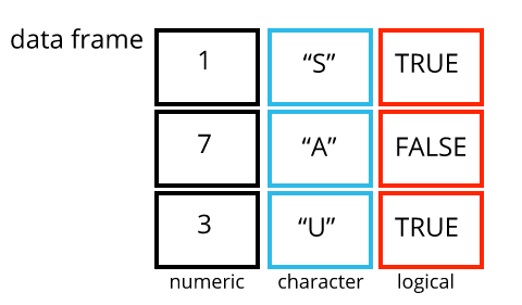
A dataframe is the representation of data in the format of a table where the columns are vectors that all have the same length. Because columns are vectors, each column must contain a single type of data (e.g., characters, integers, factors). For example, here is a figure depicting a dataframe comprising a numeric, a character, and a logical vector.

Inspect the data

You can see the contents of a dataframe by typing its name in the R console:

gapminder

# A tibble: 1,704 × 6
   country     continent  year lifeExp      pop gdpPercap
   <chr>       <chr>     <dbl>   <dbl>    <dbl>     <dbl>
 1 Afghanistan Asia       1952    28.8  8425333      779.
 2 Afghanistan Asia       1957    30.3  9240934      821.
 3 Afghanistan Asia       1962    32.0 10267083      853.
 4 Afghanistan Asia       1967    34.0 11537966      836.
 5 Afghanistan Asia       1972    36.1 13079460      740.
 6 Afghanistan Asia       1977    38.4 14880372      786.
 7 Afghanistan Asia       1982    39.9 12881816      978.
 8 Afghanistan Asia       1987    40.8 13867957      852.
 9 Afghanistan Asia       1992    41.7 16317921      649.
10 Afghanistan Asia       1997    41.8 22227415      635.
# ℹ 1,694 more rows

R gives you some useful summary information: the number of rows (1,704) and columns (6) and the type of each column (chr is character, dbl is numeric).

About the “gapminder” dataset

This dataset includes economic statistics from various countries over time, from https://gapminder.org.

The meaning of some columns is obvious (country, continent, year), but not others. Here is a short explanation of those:

• pop: Population
• lifeExp: Life expectancy (寿命)
• gdpPercap: GDP per capita (一人当たりの国内総生産)

Sort data with arrange()

First provide the name of the dataframe, then the column to sort by:

arrange(gapminder, lifeExp)

# A tibble: 1,704 × 6
   country      continent  year lifeExp     pop gdpPercap
   <chr>        <chr>     <dbl>   <dbl>   <dbl>     <dbl>
 1 Rwanda       Africa     1992    23.6 7290203      737.
 2 Afghanistan  Asia       1952    28.8 8425333      779.
 3 Gambia       Africa     1952    30    284320      485.
 4 Angola       Africa     1952    30.0 4232095     3521.
 5 Sierra Leone Africa     1952    30.3 2143249      880.
 6 Afghanistan  Asia       1957    30.3 9240934      821.
 7 Cambodia     Asia       1977    31.2 6978607      525.
 8 Mozambique   Africa     1952    31.3 6446316      469.
 9 Sierra Leone Africa     1957    31.6 2295678     1004.
10 Burkina Faso Africa     1952    32.0 4469979      543.
# ℹ 1,694 more rows

The default setting is to sort from small to large. To sort in the reverse (descending) direction, use desc():

arrange(gapminder, desc(lifeExp))

# A tibble: 1,704 × 6
   country          continent  year lifeExp       pop gdpPercap
   <chr>            <chr>     <dbl>   <dbl>     <dbl>     <dbl>
 1 Japan            Asia       2007    82.6 127467972    31656.
 2 Hong Kong, China Asia       2007    82.2   6980412    39725.
 3 Japan            Asia       2002    82   127065841    28605.
 4 Iceland          Europe     2007    81.8    301931    36181.
 5 Switzerland      Europe     2007    81.7   7554661    37506.
 6 Hong Kong, China Asia       2002    81.5   6762476    30209.
 7 Australia        Oceania    2007    81.2  20434176    34435.
 8 Spain            Europe     2007    80.9  40448191    28821.
 9 Sweden           Europe     2007    80.9   9031088    33860.
10 Israel           Asia       2007    80.7   6426679    25523.
# ℹ 1,694 more rows

You can sort on multiple columns. Ties will be sorted by the next column:

arrange(gapminder, continent, lifeExp)

# A tibble: 1,704 × 6
   country       continent  year lifeExp     pop gdpPercap
   <chr>         <chr>     <dbl>   <dbl>   <dbl>     <dbl>
 1 Rwanda        Africa     1992    23.6 7290203      737.
 2 Gambia        Africa     1952    30    284320      485.
 3 Angola        Africa     1952    30.0 4232095     3521.
 4 Sierra Leone  Africa     1952    30.3 2143249      880.
 5 Mozambique    Africa     1952    31.3 6446316      469.
 6 Sierra Leone  Africa     1957    31.6 2295678     1004.
 7 Burkina Faso  Africa     1952    32.0 4469979      543.
 8 Angola        Africa     1957    32.0 4561361     3828.
 9 Gambia        Africa     1957    32.1  323150      521.
10 Guinea-Bissau Africa     1952    32.5  580653      300.
# ℹ 1,694 more rows

Narrow down columns with select()

First provide the name of the dataframe, then the columns to select:

select(gapminder, year, country, gdpPercap)

# A tibble: 1,704 × 3
    year country     gdpPercap
   <dbl> <chr>           <dbl>
 1  1952 Afghanistan      779.
 2  1957 Afghanistan      821.
 3  1962 Afghanistan      853.
 4  1967 Afghanistan      836.
 5  1972 Afghanistan      740.
 6  1977 Afghanistan      786.
 7  1982 Afghanistan      978.
 8  1987 Afghanistan      852.
 9  1992 Afghanistan      649.
10  1997 Afghanistan      635.
# ℹ 1,694 more rows

Saving your output

Notice that although we have used several functions, gapminder is still the same:

gapminder

# A tibble: 1,704 × 6
   country     continent  year lifeExp      pop gdpPercap
   <chr>       <chr>     <dbl>   <dbl>    <dbl>     <dbl>
 1 Afghanistan Asia       1952    28.8  8425333      779.
 2 Afghanistan Asia       1957    30.3  9240934      821.
 3 Afghanistan Asia       1962    32.0 10267083      853.
 4 Afghanistan Asia       1967    34.0 11537966      836.
 5 Afghanistan Asia       1972    36.1 13079460      740.
 6 Afghanistan Asia       1977    38.4 14880372      786.
 7 Afghanistan Asia       1982    39.9 12881816      978.
 8 Afghanistan Asia       1987    40.8 13867957      852.
 9 Afghanistan Asia       1992    41.7 16317921      649.
10 Afghanistan Asia       1997    41.8 22227415      635.
# ℹ 1,694 more rows

This is because we have not saved any of the output. To do that, you need to create a new object with <-. You can call the object whatever you want, but use a name that is easy to remember:

gapminder_gdp <- select(gapminder, year, country, gdpPercap)

About pipes

During data analysis, we often need to perform several intermediate steps. It is not convenient to save the output of each since you have to think of names for each output object, and may not even use them for anything later. A better way to do this is using something called the “pipe”. The pipe is written like this: |> (some packages also write it like this: %>%).

The pipe takes the output from one function and passes it to the input of the next function. You can think of it as saying “and then”:

• Do this and then do this, and then do this…
• Do this |> do this, |> do this…

We can even use the pipe just with one function. Read the following as “start with gapminder and then select only year, country, and population”:

gapminder |> select(year, country, pop)

# A tibble: 1,704 × 3
    year country          pop
   <dbl> <chr>          <dbl>
 1  1952 Afghanistan  8425333
 2  1957 Afghanistan  9240934
 3  1962 Afghanistan 10267083
 4  1967 Afghanistan 11537966
 5  1972 Afghanistan 13079460
 6  1977 Afghanistan 14880372
 7  1982 Afghanistan 12881816
 8  1987 Afghanistan 13867957
 9  1992 Afghanistan 16317921
10  1997 Afghanistan 22227415
# ℹ 1,694 more rows

This becomes very useful when we want to do multiple steps. Read this as “start with gapminder, and then select only year, country, and population, and then arrange by year”:

gapminder |>
  select(year, country, pop) |>
  arrange(year)

# A tibble: 1,704 × 3
    year country          pop
   <dbl> <chr>          <dbl>
 1  1952 Afghanistan  8425333
 2  1952 Albania      1282697
 3  1952 Algeria      9279525
 4  1952 Angola       4232095
 5  1952 Argentina   17876956
 6  1952 Australia    8691212
 7  1952 Austria      6927772
 8  1952 Bahrain       120447
 9  1952 Bangladesh  46886859
10  1952 Belgium      8730405
# ℹ 1,694 more rows

We can make it easier to read by putting each step on its own line (the result is exactly the same, since R ignores spaces and line breaks):

gapminder |>
  select(year, country, pop) |>
  arrange(year)

# A tibble: 1,704 × 3
    year country          pop
   <dbl> <chr>          <dbl>
 1  1952 Afghanistan  8425333
 2  1952 Albania      1282697
 3  1952 Algeria      9279525
 4  1952 Angola       4232095
 5  1952 Argentina   17876956
 6  1952 Australia    8691212
 7  1952 Austria      6927772
 8  1952 Bahrain       120447
 9  1952 Bangladesh  46886859
10  1952 Belgium      8730405
# ℹ 1,694 more rows

Pipes are very useful because you don’t have to save each intermediate step. This is a very useful way to manipulate data. Therefore, the rest of the lesson will use the pipe, to help you get used to it.

Subset rows with filter()

Use the filter() function to only keep rows that meet a certain condition. For example, let’s only keep the data in Europe:

gapminder |> filter(continent == "Europe")

# A tibble: 360 × 6
   country continent  year lifeExp     pop gdpPercap
   <chr>   <chr>     <dbl>   <dbl>   <dbl>     <dbl>
 1 Albania Europe     1952    55.2 1282697     1601.
 2 Albania Europe     1957    59.3 1476505     1942.
 3 Albania Europe     1962    64.8 1728137     2313.
 4 Albania Europe     1967    66.2 1984060     2760.
 5 Albania Europe     1972    67.7 2263554     3313.
 6 Albania Europe     1977    68.9 2509048     3533.
 7 Albania Europe     1982    70.4 2780097     3631.
 8 Albania Europe     1987    72   3075321     3739.
 9 Albania Europe     1992    71.6 3326498     2497.
10 Albania Europe     1997    73.0 3428038     3193.
# ℹ 350 more rows

Modify data with mutate()

For example, we could change the units of population to millions of people:

gapminder |> mutate(pop = pop / 1000000)

# A tibble: 1,704 × 6
   country     continent  year lifeExp   pop gdpPercap
   <chr>       <chr>     <dbl>   <dbl> <dbl>     <dbl>
 1 Afghanistan Asia       1952    28.8  8.43      779.
 2 Afghanistan Asia       1957    30.3  9.24      821.
 3 Afghanistan Asia       1962    32.0 10.3       853.
 4 Afghanistan Asia       1967    34.0 11.5       836.
 5 Afghanistan Asia       1972    36.1 13.1       740.
 6 Afghanistan Asia       1977    38.4 14.9       786.
 7 Afghanistan Asia       1982    39.9 12.9       978.
 8 Afghanistan Asia       1987    40.8 13.9       852.
 9 Afghanistan Asia       1992    41.7 16.3       649.
10 Afghanistan Asia       1997    41.8 22.2       635.
# ℹ 1,694 more rows

If we provide a new column name, that column will be added

gapminder |> mutate(pop_mil = pop / 1000000)

# A tibble: 1,704 × 7
   country     continent  year lifeExp      pop gdpPercap pop_mil
   <chr>       <chr>     <dbl>   <dbl>    <dbl>     <dbl>   <dbl>
 1 Afghanistan Asia       1952    28.8  8425333      779.    8.43
 2 Afghanistan Asia       1957    30.3  9240934      821.    9.24
 3 Afghanistan Asia       1962    32.0 10267083      853.   10.3 
 4 Afghanistan Asia       1967    34.0 11537966      836.   11.5 
 5 Afghanistan Asia       1972    36.1 13079460      740.   13.1 
 6 Afghanistan Asia       1977    38.4 14880372      786.   14.9 
 7 Afghanistan Asia       1982    39.9 12881816      978.   12.9 
 8 Afghanistan Asia       1987    40.8 13867957      852.   13.9 
 9 Afghanistan Asia       1992    41.7 16317921      649.   16.3 
10 Afghanistan Asia       1997    41.8 22227415      635.   22.2 
# ℹ 1,694 more rows

Calculate summary statistics with summarize()

For example, let’s calculate the overall mean population:

gapminder |> summarize(mean_pop = mean(pop))

# A tibble: 1 × 1
   mean_pop
      <dbl>
1 29601212.

As another example, let’s calculate the total population over all the data:

gapminder |> summarize(total_pop = sum(pop))

# A tibble: 1 × 1
    total_pop
        <dbl>
1 50440465801

Use group_by() to do calculations per group

However, it is often more useful to calculate such summary statistics for particular groups. To do this, first specify the groups with group_by():

gapminder |> group_by(continent)

# A tibble: 1,704 × 6
# Groups:   continent [5]
   country     continent  year lifeExp      pop gdpPercap
   <chr>       <chr>     <dbl>   <dbl>    <dbl>     <dbl>
 1 Afghanistan Asia       1952    28.8  8425333      779.
 2 Afghanistan Asia       1957    30.3  9240934      821.
 3 Afghanistan Asia       1962    32.0 10267083      853.
 4 Afghanistan Asia       1967    34.0 11537966      836.
 5 Afghanistan Asia       1972    36.1 13079460      740.
 6 Afghanistan Asia       1977    38.4 14880372      786.
 7 Afghanistan Asia       1982    39.9 12881816      978.
 8 Afghanistan Asia       1987    40.8 13867957      852.
 9 Afghanistan Asia       1992    41.7 16317921      649.
10 Afghanistan Asia       1997    41.8 22227415      635.
# ℹ 1,694 more rows

Next, use summarize() to calculate the summary statistic:

gapminder |>
  group_by(continent) |>
  summarize(mean_pop = mean(pop))

# A tibble: 5 × 2
  continent  mean_pop
  <chr>         <dbl>
1 Africa     9916003.
2 Americas  24504795.
3 Asia      77038722.
4 Europe    17169765.
5 Oceania    8874672.

summarize() and mutate() are related since they both create new columns (or over-write existing ones). You can remember the key difference between them is that mutate() keeps the number of rows the same, whereas summarize() always decreases the number of rows.

Summary

Here is a list of the data-wrangling commands we have learned so far:

• Sort data with arrange()
• Narrow down columns with select()
• Filter rows with filter()
• Modify data with mutate()
• Summarize data with summarize()
• Group data with group_by()

By combining these functions, each of which is fairly simple, with the pipe (|>), you can construct sophisticated data analysis pipelines.

Submitting the homework

Go to Moodle, click on the Day 4 Homework assignment, and click on the link to accept the assignment. This will create the repo in your GitHub account.

Next, clone the remote repo to your local machine. Then, edit the file day_04_homework.R file in RStudio. Make sure that your code runs without errors. Once you have done so, commit your changes and push to the remote. Don’t forget to push! If you don’t push, your work will not be submitted.

You can double check that you’ve successfully submitted (pushed) the homework by visiting your GitHub repo in your browser (use the same link in Moodle that you clicked to accept the assignment). Make sure the homework file there shows the same changes that you made in RStudio.

Be sure to do this BY THE DEADLINE, or your work will not be counted.

Attributions

These materials were modified by Joel H. Nitta from those posted at https://swcarpentry.github.io/r-novice-gapminder/ and https://datacarpentry.org/R-ecology-lesson under the Creative Commons Attribution (CC BY 4.0) license.