Day 5: Joining Data

Overview

• So far, we have been working with a single dataframe

• But sometimes, data comes to us as multiple dataframes

  • This is also known as a “database”

• We will learn how to join data across dataframes

Recommended Reading

Hadely Wickham, R for Data Science (2e)

• Chapter 19, “Joins”

Set up

• We will continue to use the gapminder-analysis project in the data-analysis-course folder on your Desktop
  • This is actually a different dataset, so the name for the project isn’t ideal. Naming things is hard!
• Create a new file in that project called joining-practice.R
  • We will save all the demonstration code in that script

• Be sure to follow along! (don’t just watch the video without running the code)

• We will use data in the nycflights13 package to demonstrate joins, so install that first (remember you only need to install a package once, so don’t include this in your code)

install.packages("nycflights13")

• The first thing to do in our script is to load the necessary packages:

joining-practice.R

library(tidyverse)
library(nycflights13)

About the nycflights13 data

• The main dataframe in nycflights13 is called flights and includes data about flights that departed from New York in 2013

https://www.express.co.uk/travel/articles/1440362/us-holidays-jetblue-flights-travel-low-cost-budget-heathrow-gatwick

About the nycflights13 data

• You can read the helpfile with ?flights

• You can view it by typing flights:

flights

# A tibble: 336,776 × 19
   year month   day dep_time sched_dep_time dep_delay arr_time sched_arr_time
  <int> <int> <int>    <int>          <int>     <dbl>    <int>          <int>
1  2013     1     1      517            515         2      830            819
2  2013     1     1      533            529         4      850            830
3  2013     1     1      542            540         2      923            850
4  2013     1     1      544            545        -1     1004           1022
5  2013     1     1      554            600        -6      812            837
6  2013     1     1      554            558        -4      740            728
# ℹ 336,770 more rows
# ℹ 11 more variables: arr_delay <dbl>, carrier <chr>, flight <int>,
#   tailnum <chr>, origin <chr>, dest <chr>, air_time <dbl>, distance <dbl>,
#   hour <dbl>, minute <dbl>, time_hour <dttm>

About the nycflights13 data

• The package also includes several other related dataframes:
  • weather: hourly meterological data for each airport
  • planes: construction information about each plane
  • airports: airport names and locations
  • airlines: translation between two letter carrier codes and airline names
• We can read the helpfile for each one and view it in the same way as flights (for example, ?weather)

About keys

• Dataframes often include a special column called the primary key

• The values of the primary key are unique to each row. In other words, we can identify a row using the primary key.

• The primary key is often the first column in the data, but not always

About keys

• Let’s look at an example. The primary key for planes is tailnum
  • The “tail number” is a unique code on the tail of each airplane

https://www.quora.com/Is-there-a-general-name-for-the-identifying-numbers-on-the-sides-of-airplanes

About keys: planes

planes

# A tibble: 3,322 × 9
  tailnum  year type               manufacturer model engines seats speed engine
  <chr>   <int> <chr>              <chr>        <chr>   <int> <int> <int> <chr> 
1 N10156   2004 Fixed wing multi … EMBRAER      EMB-…       2    55    NA Turbo…
2 N102UW   1998 Fixed wing multi … AIRBUS INDU… A320…       2   182    NA Turbo…
3 N103US   1999 Fixed wing multi … AIRBUS INDU… A320…       2   182    NA Turbo…
4 N104UW   1999 Fixed wing multi … AIRBUS INDU… A320…       2   182    NA Turbo…
5 N10575   2002 Fixed wing multi … EMBRAER      EMB-…       2    55    NA Turbo…
6 N105UW   1999 Fixed wing multi … AIRBUS INDU… A320…       2   182    NA Turbo…
# ℹ 3,316 more rows

About keys: planes

Notice that the values of tailnum appear unique, while the values of other columns may be repeated.

But we should actually check this…

Verifying the primary key

We can verify that the primary is indeed unique by counting how many times each tailnum occurs in planes:

planes |>
  count(tailnum)

# A tibble: 3,322 × 2
  tailnum     n
  <chr>   <int>
1 N10156      1
2 N102UW      1
3 N103US      1
4 N104UW      1
5 N10575      1
6 N105UW      1
# ℹ 3,316 more rows

Verifying the primary key

What we are really concerned with, is whether any tail number occurs more than once. Let’s check that with filter:

planes |>
  count(tailnum) |>
  filter(n > 1)

# A tibble: 0 × 2
# ℹ 2 variables: tailnum <chr>, n <int>

Good!

Verifying the primary key

Another important thing to check is missing values. We can’t identify a row if its identifier is missing!

planes |>
  filter(is.na(tailnum))

# A tibble: 0 × 9
# ℹ 9 variables: tailnum <chr>, year <int>, type <chr>, manufacturer <chr>,
#   model <chr>, engines <int>, seats <int>, speed <int>, engine <chr>

Also good!

Primary keys of other dataframes

• OK, so we know the primary key of planes is tailnum.

• What about the other dataframes?

airports

The primary key of airports is its three-letter airport code, which is named in the the dataframe faa:

airports

# A tibble: 1,458 × 8
  faa   name                             lat   lon   alt    tz dst   tzone      
  <chr> <chr>                          <dbl> <dbl> <dbl> <dbl> <chr> <chr>      
1 04G   Lansdowne Airport               41.1 -80.6  1044    -5 A     America/Ne…
2 06A   Moton Field Municipal Airport   32.5 -85.7   264    -6 A     America/Ch…
3 06C   Schaumburg Regional             42.0 -88.1   801    -6 A     America/Ch…
4 06N   Randall Airport                 41.4 -74.4   523    -5 A     America/Ne…
5 09J   Jekyll Island Airport           31.1 -81.4    11    -5 A     America/Ne…
6 0A9   Elizabethton Municipal Airport  36.4 -82.2  1593    -5 A     America/Ne…
# ℹ 1,452 more rows

Challenge: Check the key

But (like I mentioned before) it’s a good idea to verify that faa is indeed a valid primary key! Can you do it?

Compound keys

• Sometimes, no single column is provided as a key. Instead, multiple columns may be combined that uniquely identify each row.

• For example, in the weather dataframe, the combination of origin and time_hour combined are unique.

weather

# A tibble: 26,115 × 15
  origin  year month   day  hour  temp  dewp humid wind_dir wind_speed wind_gust
  <chr>  <int> <int> <int> <int> <dbl> <dbl> <dbl>    <dbl>      <dbl>     <dbl>
1 EWR     2013     1     1     1  39.0  26.1  59.4      270      10.4         NA
2 EWR     2013     1     1     2  39.0  27.0  61.6      250       8.06        NA
3 EWR     2013     1     1     3  39.0  28.0  64.4      240      11.5         NA
4 EWR     2013     1     1     4  39.9  28.0  62.2      250      12.7         NA
5 EWR     2013     1     1     5  39.0  28.0  64.4      260      12.7         NA
6 EWR     2013     1     1     6  37.9  28.0  67.2      240      11.5         NA
# ℹ 26,109 more rows
# ℹ 4 more variables: precip <dbl>, pressure <dbl>, visib <dbl>,
#   time_hour <dttm>

• This is a bit easier to see if we rearrange the columns:

weather |>
  relocate(time_hour, .after = 1)

# A tibble: 26,115 × 15
  origin time_hour            year month   day  hour  temp  dewp humid wind_dir
  <chr>  <dttm>              <int> <int> <int> <int> <dbl> <dbl> <dbl>    <dbl>
1 EWR    2013-01-01 01:00:00  2013     1     1     1  39.0  26.1  59.4      270
2 EWR    2013-01-01 02:00:00  2013     1     1     2  39.0  27.0  61.6      250
3 EWR    2013-01-01 03:00:00  2013     1     1     3  39.0  28.0  64.4      240
4 EWR    2013-01-01 04:00:00  2013     1     1     4  39.9  28.0  62.2      250
5 EWR    2013-01-01 05:00:00  2013     1     1     5  39.0  28.0  64.4      260
6 EWR    2013-01-01 06:00:00  2013     1     1     6  37.9  28.0  67.2      240
# ℹ 26,109 more rows
# ℹ 5 more variables: wind_speed <dbl>, wind_gust <dbl>, precip <dbl>,
#   pressure <dbl>, visib <dbl>

Verify the compound key

• We can also verify a compound key, much like before.
  • This time, we need to add group_by() before counting:

weather |>
  group_by(origin, time_hour) |>
  count() |>
  filter(n > 1)

# A tibble: 0 × 3
# Groups:   origin, time_hour [0]
# ℹ 3 variables: origin <chr>, time_hour <dttm>, n <int>

Good!

Keys are used to match dataframes

• The reason we care about keys is that they can be used to link dataframes

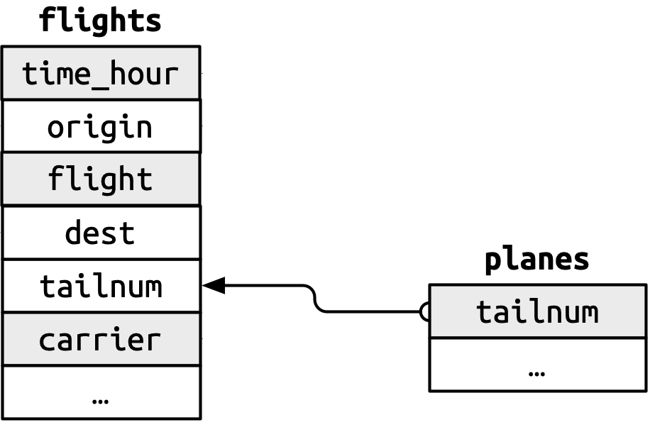
• For example, look at some of the data in flights
  • Notice the column tailnum?
  • tailnum is not unique in flights (it is not a key in that dataframe), but it can be linked to the planes dataframe
  • This allows us to find out more information about each plane in the flights data

• In the context of planes, tailnum is the primary key
• In the context of flights, tailnum is called a “foreign key” (it corresponds to a primary key in a different dataframe)

Summary of keys in nycflights13

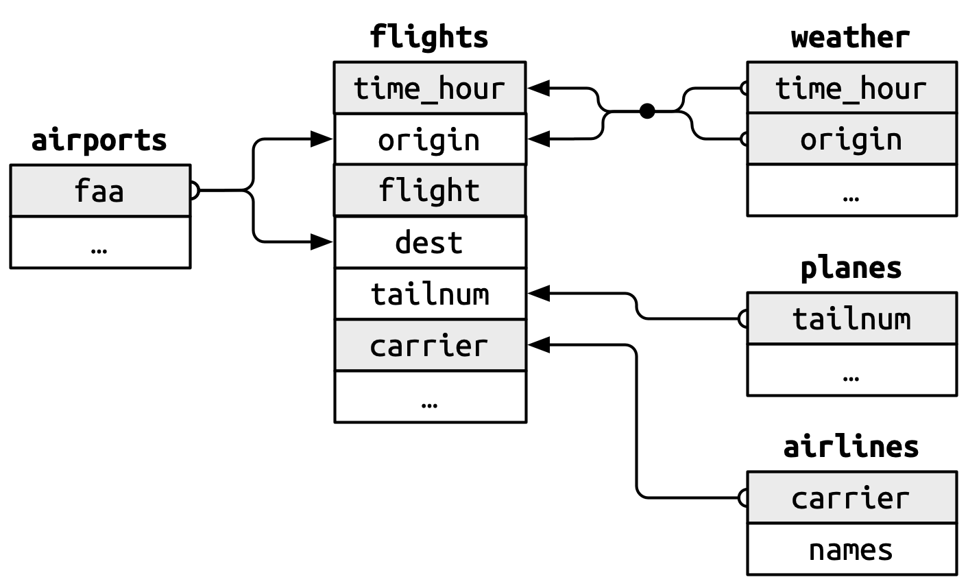
Variables making up a primary key are colored grey, and are connected to their corresponding foreign keys with arrows.

Summary of keys

• A primary key in one dataframe is a foreign key in another dataframe

• Also notice that a given column may have different names in different dataframes (compare faa of the airports dataframe to origin of the flights dataframe)

Types of joins

• Now that we understand the theory behind joining (you need keys!), we can learn about joining functions. There are two main kinds:
  • Mutating joins add new columns to a dataframe (like the mutate() function)
  • Filtering joins filter the rows of a dataframe (like the filter() function)
• We will start with mutating joins.

Make a smaller demo dataset

• Mutating joins add columns to the right side, so they may be hard to see if your dataframe already has many columns.

• Let’s make a smaller one called flights2 for demo purposes:

flights2 <- flights |>
  select(year, time_hour, origin, dest, tailnum, carrier)

flights2

# A tibble: 336,776 × 6
   year time_hour           origin dest  tailnum carrier
  <int> <dttm>              <chr>  <chr> <chr>   <chr>  
1  2013 2013-01-01 05:00:00 EWR    IAH   N14228  UA     
2  2013 2013-01-01 05:00:00 LGA    IAH   N24211  UA     
3  2013 2013-01-01 05:00:00 JFK    MIA   N619AA  AA     
4  2013 2013-01-01 05:00:00 JFK    BQN   N804JB  B6     
5  2013 2013-01-01 06:00:00 LGA    ATL   N668DN  DL     
6  2013 2013-01-01 05:00:00 EWR    ORD   N39463  UA     
# ℹ 336,770 more rows

left_join()

• The most frequently used join
  • Adds new columns to the dataframe you’re joining to
• For example, add the airline carrier name to the flights data:

flights2 |>
  left_join(airlines)

# A tibble: 336,776 × 7
   year time_hour           origin dest  tailnum carrier name                  
  <int> <dttm>              <chr>  <chr> <chr>   <chr>   <chr>                 
1  2013 2013-01-01 05:00:00 EWR    IAH   N14228  UA      United Air Lines Inc. 
2  2013 2013-01-01 05:00:00 LGA    IAH   N24211  UA      United Air Lines Inc. 
3  2013 2013-01-01 05:00:00 JFK    MIA   N619AA  AA      American Airlines Inc.
4  2013 2013-01-01 05:00:00 JFK    BQN   N804JB  B6      JetBlue Airways       
5  2013 2013-01-01 06:00:00 LGA    ATL   N668DN  DL      Delta Air Lines Inc.  
6  2013 2013-01-01 05:00:00 EWR    ORD   N39463  UA      United Air Lines Inc. 
# ℹ 336,770 more rows

Challenge: join the weather data

Let’s say we want to know more about the weather on the day of each flight.

How can we join the weather data to the flight data?

Specifying the key

• You may have noticed a message like this in the output:

Joining with `by = join_by(carrier)`

• That is because we did not specify how to join the data (which keys are the primary and foreign keys), so it guessed.

• By default, left_join() will join on column names that are in common between both dataframes.

• But, the default settings do not always work well

• For example:

flights2 |>
  left_join(planes)

# A tibble: 336,776 × 13
   year time_hour           origin dest  tailnum carrier type  manufacturer
  <int> <dttm>              <chr>  <chr> <chr>   <chr>   <chr> <chr>       
1  2013 2013-01-01 05:00:00 EWR    IAH   N14228  UA      <NA>  <NA>        
2  2013 2013-01-01 05:00:00 LGA    IAH   N24211  UA      <NA>  <NA>        
3  2013 2013-01-01 05:00:00 JFK    MIA   N619AA  AA      <NA>  <NA>        
4  2013 2013-01-01 05:00:00 JFK    BQN   N804JB  B6      <NA>  <NA>        
5  2013 2013-01-01 06:00:00 LGA    ATL   N668DN  DL      <NA>  <NA>        
6  2013 2013-01-01 05:00:00 EWR    ORD   N39463  UA      <NA>  <NA>        
# ℹ 336,770 more rows
# ℹ 5 more variables: model <chr>, engines <int>, seats <int>, speed <int>,
#   engine <chr>

NA indicates that the data from planes are missing (could not be matched)… why are so many rows missing data??

• The problem is that year has a different meaning in flights and planes
  • planes: year is the year the plane was built
  • flights: year is the year of the flight
• We can avoid this problem by specifying how to join the data with join_by()

flights2 |>
  left_join(planes, join_by(tailnum))

# A tibble: 336,776 × 14
  year.x time_hour           origin dest  tailnum carrier year.y type           
   <int> <dttm>              <chr>  <chr> <chr>   <chr>    <int> <chr>          
1   2013 2013-01-01 05:00:00 EWR    IAH   N14228  UA        1999 Fixed wing mul…
2   2013 2013-01-01 05:00:00 LGA    IAH   N24211  UA        1998 Fixed wing mul…
3   2013 2013-01-01 05:00:00 JFK    MIA   N619AA  AA        1990 Fixed wing mul…
4   2013 2013-01-01 05:00:00 JFK    BQN   N804JB  B6        2012 Fixed wing mul…
5   2013 2013-01-01 06:00:00 LGA    ATL   N668DN  DL        1991 Fixed wing mul…
6   2013 2013-01-01 05:00:00 EWR    ORD   N39463  UA        2012 Fixed wing mul…
# ℹ 336,770 more rows
# ℹ 6 more variables: manufacturer <chr>, model <chr>, engines <int>,
#   seats <int>, speed <int>, engine <chr>

Notice that the output has year.x and year.y, indicating the year column that came from each dataframe

• Actually, join_by(tailnum) is short for join_by(tailnum == tailnum)
  • In this case, we are joining by the same column name on the left and the right side (both dataframes)

flights2 |>
  left_join(planes, join_by(tailnum == tailnum))

# A tibble: 336,776 × 14
  year.x time_hour           origin dest  tailnum carrier year.y type           
   <int> <dttm>              <chr>  <chr> <chr>   <chr>    <int> <chr>          
1   2013 2013-01-01 05:00:00 EWR    IAH   N14228  UA        1999 Fixed wing mul…
2   2013 2013-01-01 05:00:00 LGA    IAH   N24211  UA        1998 Fixed wing mul…
3   2013 2013-01-01 05:00:00 JFK    MIA   N619AA  AA        1990 Fixed wing mul…
4   2013 2013-01-01 05:00:00 JFK    BQN   N804JB  B6        2012 Fixed wing mul…
5   2013 2013-01-01 06:00:00 LGA    ATL   N668DN  DL        1991 Fixed wing mul…
6   2013 2013-01-01 05:00:00 EWR    ORD   N39463  UA        2012 Fixed wing mul…
# ℹ 336,770 more rows
# ℹ 6 more variables: manufacturer <chr>, model <chr>, engines <int>,
#   seats <int>, speed <int>, engine <chr>

• But it is useful to be able to specify different column names when joining.

• For example, when we join the airports data

• Join by the destination airport:

flights2 |>
  left_join(airports, join_by(dest == faa))

# A tibble: 336,776 × 13
   year time_hour           origin dest  tailnum carrier name    lat   lon   alt
  <int> <dttm>              <chr>  <chr> <chr>   <chr>   <chr> <dbl> <dbl> <dbl>
1  2013 2013-01-01 05:00:00 EWR    IAH   N14228  UA      Geor…  30.0 -95.3    97
2  2013 2013-01-01 05:00:00 LGA    IAH   N24211  UA      Geor…  30.0 -95.3    97
3  2013 2013-01-01 05:00:00 JFK    MIA   N619AA  AA      Miam…  25.8 -80.3     8
4  2013 2013-01-01 05:00:00 JFK    BQN   N804JB  B6      <NA>   NA    NA      NA
5  2013 2013-01-01 06:00:00 LGA    ATL   N668DN  DL      Hart…  33.6 -84.4  1026
6  2013 2013-01-01 05:00:00 EWR    ORD   N39463  UA      Chic…  42.0 -87.9   668
# ℹ 336,770 more rows
# ℹ 3 more variables: tz <dbl>, dst <chr>, tzone <chr>

• Join by the originating airport:

flights2 |>
  left_join(airports, join_by(origin == faa))

# A tibble: 336,776 × 13
   year time_hour           origin dest  tailnum carrier name    lat   lon   alt
  <int> <dttm>              <chr>  <chr> <chr>   <chr>   <chr> <dbl> <dbl> <dbl>
1  2013 2013-01-01 05:00:00 EWR    IAH   N14228  UA      Newa…  40.7 -74.2    18
2  2013 2013-01-01 05:00:00 LGA    IAH   N24211  UA      La G…  40.8 -73.9    22
3  2013 2013-01-01 05:00:00 JFK    MIA   N619AA  AA      John…  40.6 -73.8    13
4  2013 2013-01-01 05:00:00 JFK    BQN   N804JB  B6      John…  40.6 -73.8    13
5  2013 2013-01-01 06:00:00 LGA    ATL   N668DN  DL      La G…  40.8 -73.9    22
6  2013 2013-01-01 05:00:00 EWR    ORD   N39463  UA      Newa…  40.7 -74.2    18
# ℹ 336,770 more rows
# ℹ 3 more variables: tz <dbl>, dst <chr>, tzone <chr>

Other mutating joins

*_join(x, y)

• left_join(x, y): keep all rows in x
• right_join(x, y): keep all rows in y
• inner_join(x, y): keep only rows in common between x and y
• full_join(x, y): keep all rows in both x and y

We don’t have time to cover them in detail, but please try them out!

Filtering joins

• Filtering joins are different from mutating joins in that they do not add new data

• Instead, we only use them to filter data

semi_join()

• semi_join(x, y): Keep all rows in x that have a match in y

Use a semi-join to filter the airports dataset to show just the airports where the flights originated from (there are three airports in NYC):

airports |>
  semi_join(flights2, join_by(faa == origin))

# A tibble: 3 × 8
  faa   name                  lat   lon   alt    tz dst   tzone           
  <chr> <chr>               <dbl> <dbl> <dbl> <dbl> <chr> <chr>           
1 EWR   Newark Liberty Intl  40.7 -74.2    18    -5 A     America/New_York
2 JFK   John F Kennedy Intl  40.6 -73.8    13    -5 A     America/New_York
3 LGA   La Guardia           40.8 -73.9    22    -5 A     America/New_York

anti_join()

• anti_join(x, y): Keep all rows in x that don’t have a match in y

• Useful to check for implicit missing data

Find rows that are missing from airports by looking for flights that don’t have a matching destination airport:

flights2 |>
  anti_join(airports, join_by(dest == faa)) |>
  distinct(dest)

# A tibble: 4 × 1
  dest 
  <chr>
1 BQN  
2 SJU  
3 STT  
4 PSE  

Summary

• Keys are columns that we use to join dataframes

• Mutating joins add columns to a dataframe

• Filtering joins filter the rows of a dataframe

Knowing how to join data will greatly expand the kinds of data analysis you can do. Now you are not limited to a single dataframe, but have the ability to combine dataframes together as needed.