Reproducible Data Analysis Day 6: Data visualization with ggplot2
Learning Objectives
By the end of this class, you should be able to do the following:
Use ggplot2 to generate publication-quality graphics.
Apply geometry and aesthetic layers to a ggplot plot.
Manipulate the aesthetics of a plot using different colors, shapes, and lines.
Improve data visualization through transforming scales and paneling by group.
Save a plot created with ggplot to disk.
About plotting and ggplot2
Plotting our data is one of the best ways to quickly explore it and the various relationships between variables.
Today we’ll be learning about the ggplot2 package, because it has a consistent syntax and can be used to produce publication-quality graphics.
We do not have time to cover nearly everything there is to know about ggplot2. For more information, I highly recommend the book written by the author of ggplot2, Hadley Wickham: ggplot2: Elegant Graphics for Data Analysis.
ggplot2 is built on the grammar of graphics, the idea that any plot can be built from the same set of components: a data set, mapping aesthetics, and graphical layers:
Data sets are the data that you, the user, provide.
Mapping aesthetics are what connect the data to the graphics. They tell ggplot2 how to use your data to affect how the graph looks, such as changing what is plotted on the X or Y axis, or the size or color of different data points.
Layers are the actual graphical output from ggplot2. Layers determine what kinds of plot are shown (scatterplot, histogram, etc.), the coordinate system used (rectangular, polar, others), and other important aspects of the plot. The idea of layers of graphics may be familiar to you if you have used image editing programs like Photoshop, Illustrator, or Inkscape.
Let’s start off building an example using the gapminder data from earlier. The most basic function is ggplot, which lets R know that we’re creating a new plot. Any of the arguments we give the ggplot function are the global options for the plot: they apply to all layers on the plot.
Getting started
Today we will continue using the local project that you created before, gapminder-analysis, located in the data-analysis-course folder on your Desktop. Open it by clicking on the gapminder-analysis.Rproj file.
Since ggplot2 is included in tidyverse, we will first load the tidyverse set of packages. Also load the scales package, which is used for labeling plots.
library(tidyverse)
── Attaching core tidyverse packages ──────────────────────── tidyverse 2.0.0 ──
✔ dplyr     1.2.1     ✔ readr     2.2.0
✔ forcats   1.0.1     ✔ stringr   1.6.0
✔ ggplot2   4.0.3     ✔ tibble    3.3.1
✔ lubridate 1.9.5     ✔ tidyr     1.3.2
✔ purrr     1.2.2
── Conflicts ────────────────────────────────────────── tidyverse_conflicts() ──
✖ dplyr::filter() masks stats::filter()
✖ dplyr::lag()    masks stats::lag()
ℹ Use the conflicted package (<http://conflicted.r-lib.org/>) to force all conflicts to become errors
library(scales)
Attaching package: 'scales'

The following object is masked from 'package:purrr':

    discard

The following object is masked from 'package:readr':

    col_factor
Next, load the data as before.
gapminder <-read_csv("data_raw/gapminder.csv")
Rows: 1704 Columns: 6
── Column specification ────────────────────────────────────────────────────────
Delimiter: ","
chr (2): country, continent
dbl (4): year, lifeExp, pop, gdpPercap

ℹ Use `spec()` to retrieve the full column specification for this data.
ℹ Specify the column types or set `show_col_types = FALSE` to quiet this message.
We are now ready to plot the data.
First plot
Let’s start off building an example using the gapminder data from earlier. The most basic function is ggplot, which lets R know that we’re creating a new plot. Any of the arguments we give the ggplot function are the global options for the plot: they apply to all layers on the plot.
ggplot(data = gapminder)
Here we called ggplot and told it what data we want to show on our figure. This is not enough information for ggplot to actually draw anything. It only creates a blank slate for other elements to be added to.
Now we’re going to add in the mapping aesthetics using the aes function. aes tells ggplot how variables in the data map to aesthetic properties of the figure, such as which columns of the data should be used for the x and y locations.
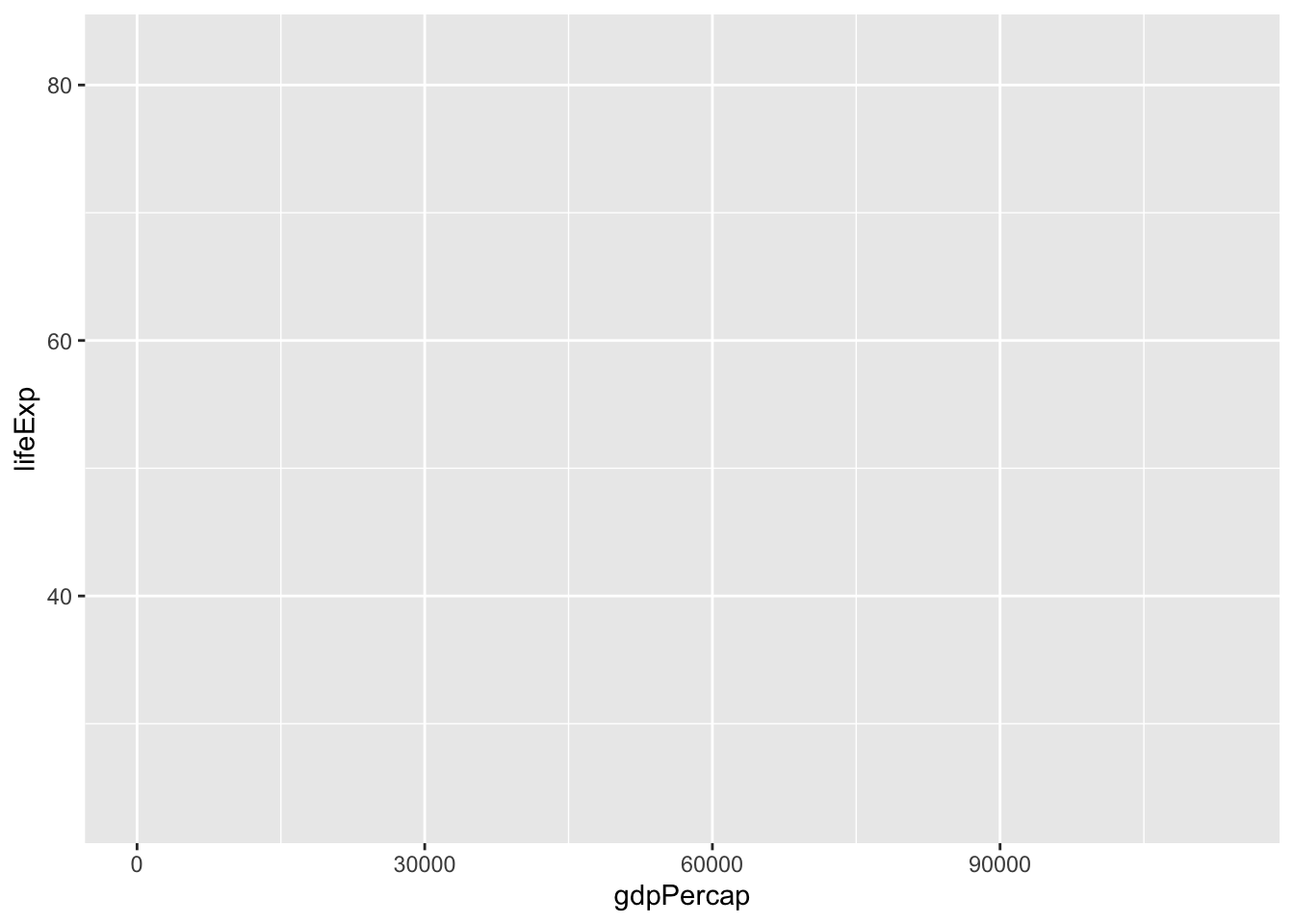
ggplot(data = gapminder, mapping =aes(x = gdpPercap, y = lifeExp))
Here we told ggplot we want to plot the “gdpPercap” column of the gapminder data frame on the x-axis, and the “lifeExp” column on the y-axis. Notice that we didn’t need to explicitly pass aes these columns (e.g. x = gapminder[, "gdpPercap"]), this is because ggplot is smart enough to know to look in the data for that column!
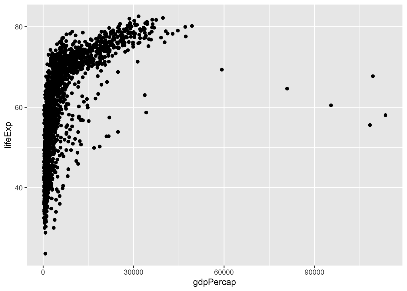
The final part of making our plot is to tell ggplot how we want to visually represent the data. We do this by adding a new layer to the plot using one of the geom functions.
Here we used geom_point, which tells ggplot we want to visually represent the relationship between x and y as a scatterplot of points.
Layers
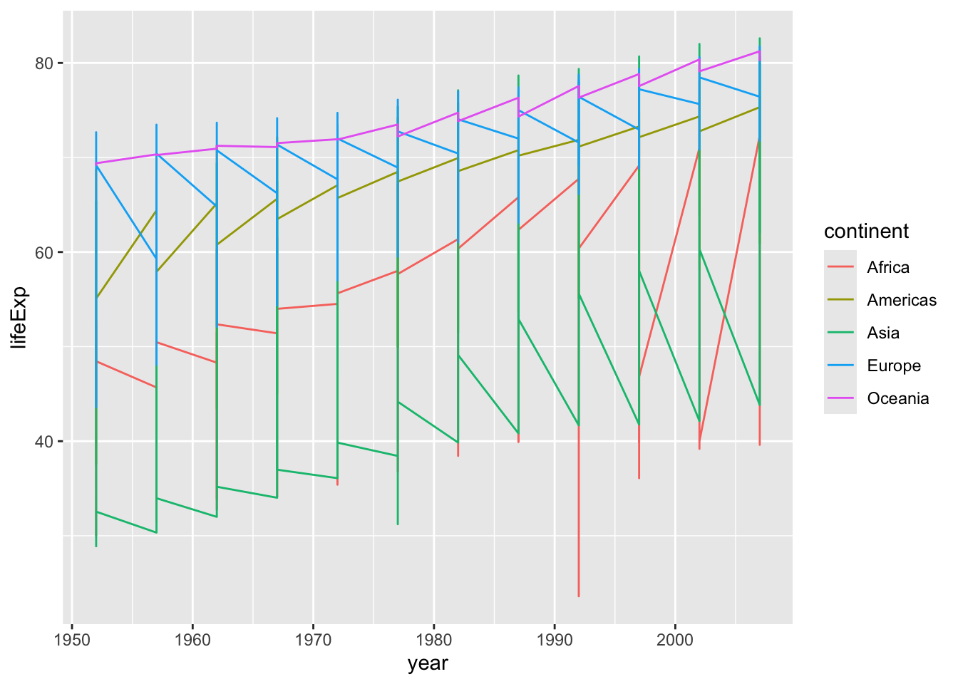
Using a scatterplot probably isn’t the best for visualizing change over time. Instead, let’s tell ggplot to visualize the data as a line plot:
ggplot(data = gapminder, mapping =aes(x = year, y = lifeExp, color = continent)) +geom_line()
Instead of adding a geom_point layer, we’ve added a geom_line layer.
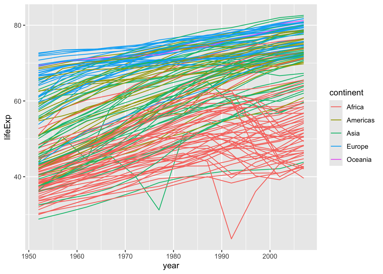
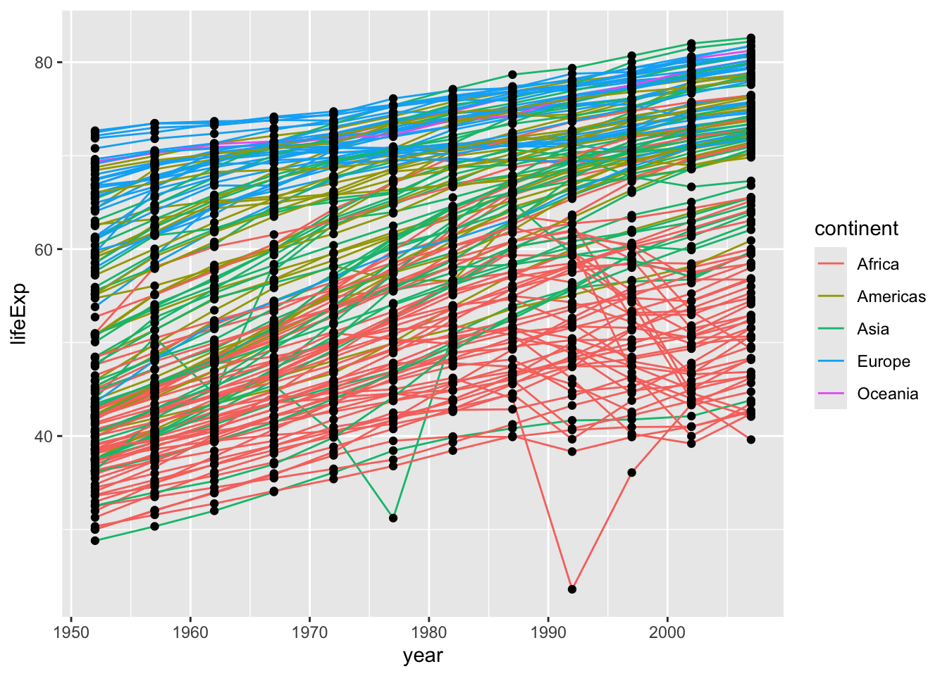
However, the result doesn’t look quite as we might have expected: it seems to be jumping around a lot in each continent. Let’s try to separate the data by country, plotting one line for each country:
ggplot(data = gapminder, mapping =aes(x = year, y = lifeExp, group = country, color = continent)) +geom_line()
We’ve added the groupaesthetic, which tells ggplot to draw a line for each country.
But what if we want to visualize both lines and points on the plot? We can add another layer to the plot:
ggplot(data = gapminder, mapping =aes(x = year, y = lifeExp, group = country, color = continent)) +geom_line() +geom_point()
It’s important to note that each layer is drawn on top of the previous layer. In this example, the points have been drawn on top of the lines. Here’s a demonstration:
ggplot(data = gapminder, mapping =aes(x = year, y = lifeExp, group = country)) +geom_line(mapping =aes(color = continent)) +geom_point()
In this example, the aesthetic mapping of color has been moved from the global plot options in ggplot to the geom_line layer so it no longer applies to the points. Now we can clearly see that the points are drawn on top of the lines.
Tip: Setting an aesthetic to a value instead of a mapping
So far, we’ve seen how to use an aesthetic (such as color) as a mapping to a variable in the data. For example, when we use geom_line(mapping = aes(color=continent)), ggplot will give a different color to each continent. But what if we want to change the color of all lines to blue? You may think that geom_line(mapping = aes(color="blue")) should work, but it doesn’t. Since we don’t want to create a mapping to a specific variable, we can move the color specification outside of the aes() function, like this: geom_line(color="blue").
Transformations
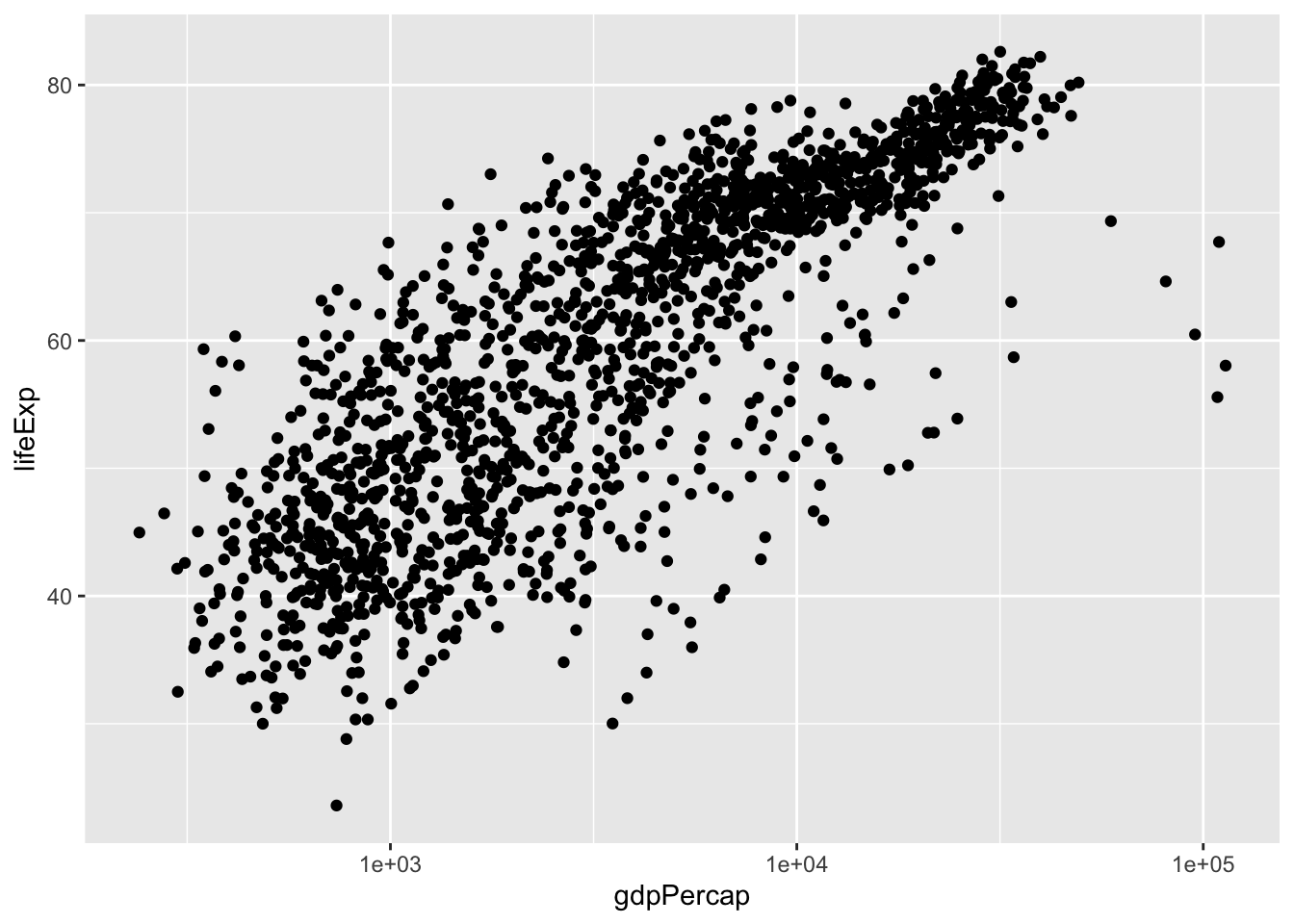
Currently it’s hard to see the relationship between the points due to some strong outliers in GDP per capita. We can change the scale of units on the x axis using the scale functions. These control the mapping between the data values and visual values of an aesthetic. We can also modify the transparency of the points, using the alpha function, which is especially helpful when you have a large amount of data which is very clustered.
The scale_x_log10 function applied a transformation to the coordinate system of the plot, so that each multiple of 10 is evenly spaced from left to right. For example, a GDP per capita of 1,000 is the same horizontal distance away from a value of 10,000 as the 10,000 value is from 100,000. This helps to visualize the spread of the data along the x-axis.
You may not be used to reading scientific notation. We can change the way the labels on the x-axis appear using the labels argument of the scale_x_log10() function:
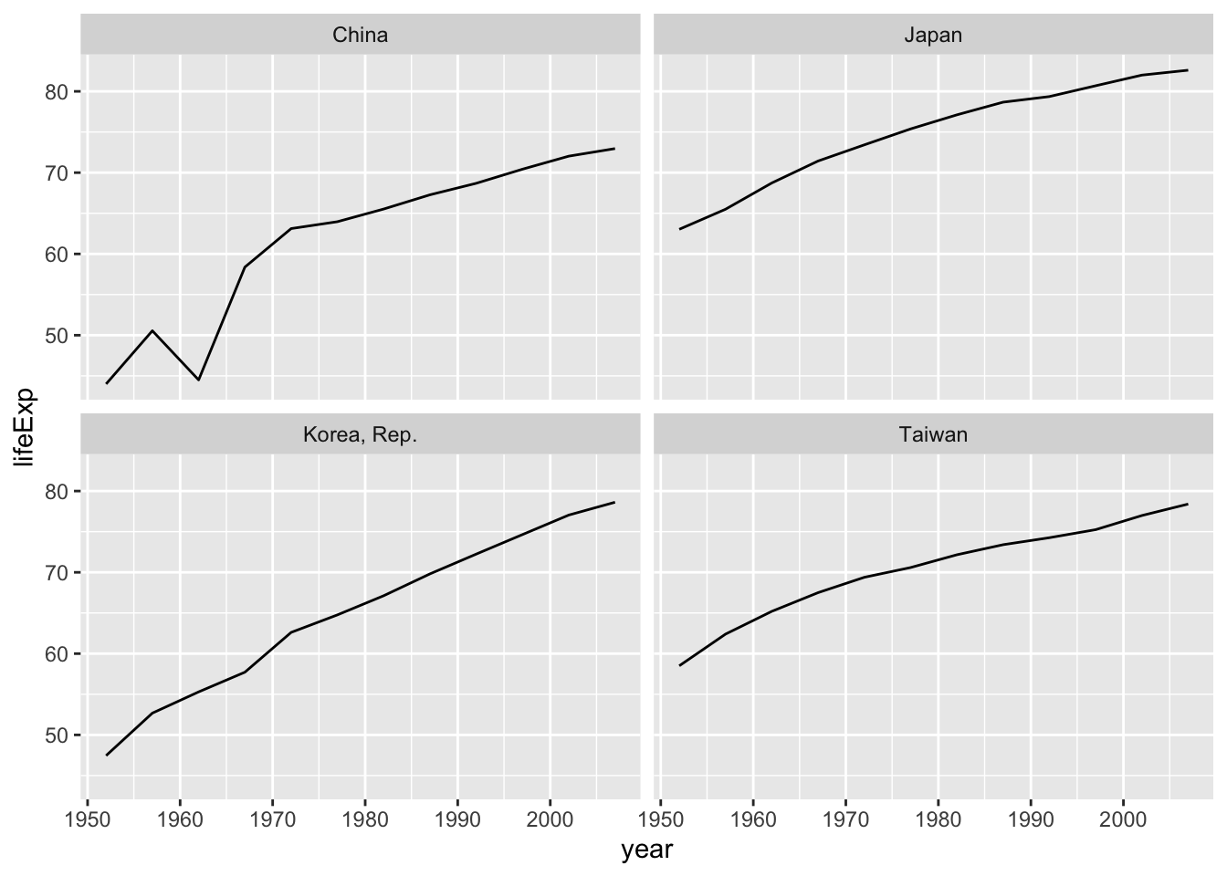
Earlier we visualized the change in life expectancy over time across all countries in one plot. Alternatively, we can split this out over multiple panels by adding a layer of facet panels.
We start by making a subset of data including only some countries located in Asia. (Otherwise, there are too many countries to plot).
gapminder_asia <-filter( gapminder, country %in%c("Japan", "China", "Korea, Rep.", "Taiwan"))
Use facet_wrap() to create the facets. Note that within facet_wrap(), you need to specify the variable to use for grouping the facets with vars(). Here, we group the facets by country; in other words, each facet is one country.
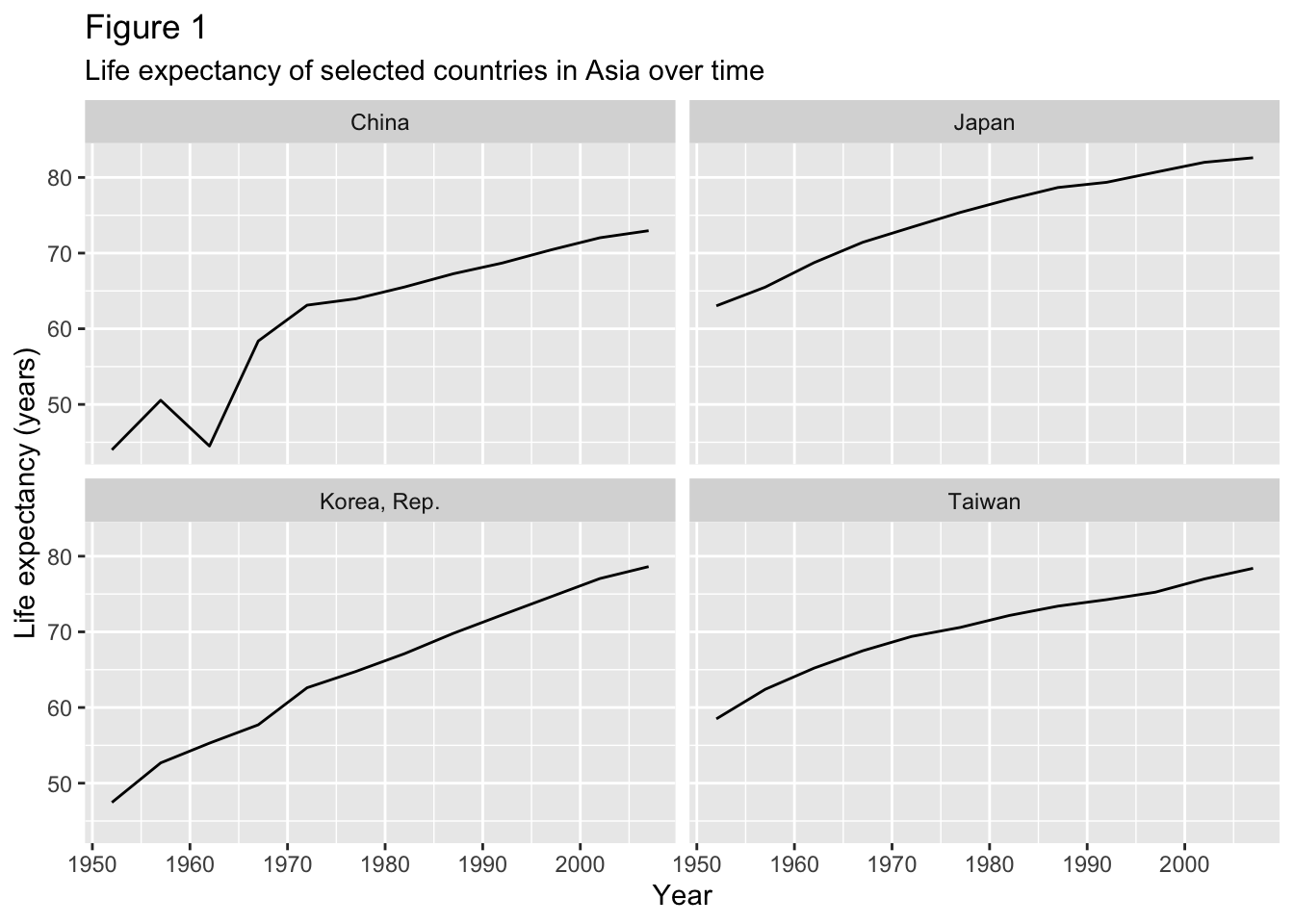
To clean this figure up for a publication we need to change some of the labels. The y axis should read “Life expectancy”, rather than the column name in the data frame. It’s also a good idea to indicate the units of the data (years for life expectancy).
You can change these using the labs() function. You set the value of each label as a character string (for example, x = "Year", etc.):
ggplot( gapminder_asia,aes(x = year,y = lifeExp )) +geom_line() +facet_wrap(vars(country)) +labs(x ="Year", # x axis titley ="Life expectancy (years)", # y axis titletitle ="Figure 1", # main title of figuresubtitle ="Life expectancy of selected countries in Asia over time" )
Exporting the plot
First, re-run the code above, and save the output in R to an object, which we will call gapminder_asia_plot.
gapminder_asia_plot <-ggplot( gapminder_asia,aes(x = year,y = lifeExp )) +geom_line() +facet_wrap(vars(country)) +labs(x ="Year",y ="Life expectancy (years)",title ="Figure 1",subtitle ="Life expectancy of selected countries in Asia over time" )
Next, use the ggsave() function to export the plot to a file. You can specify the dimension and resolution of your plot by adjusting the appropriate arguments (width, height and dpi) to create high quality graphics for publication. In order to save the plot from above, we first assign it to a variable lifeExp_plot, then tell ggsave to save that plot in pdf format. You can also specify other formats like pdf or jpg.
As a general rule, you should not commit the output of code to your repository. That is because you can reproduce the output from the code (which you should commit) and the data (which is read-only). Best practice is to create a folder for storing results called results/, and add this folder to your .gitignore so that anything that it contains will be excluded from your git repo.
To save the above plot to the results folder, modify the file argument to look like this (make sure to create results first!):