Loading data from TidyTuesday

TidyTuesday is a GitHub repo that provides one dataset per week to practice learning data science skills.

For the final project, you will choose one dataset from TidyTuesday and use it to make at least two plots.

This will show you how to find and load a dataset from TidyTuesday.

Choose a dataset

In your browser, navigate to https://github.com/rfordatascience/tidytuesday

TidyTuesday repo

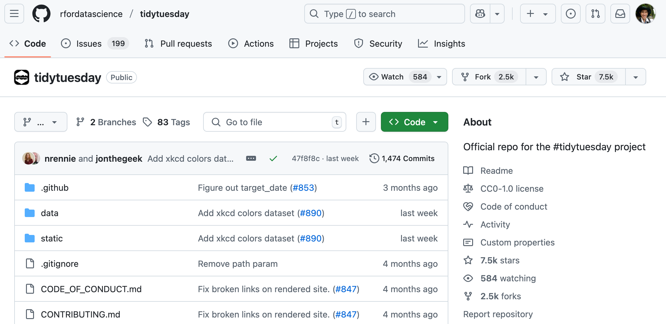
Scroll down until you reach the section labeled “DataSets”.

“DataSets” section

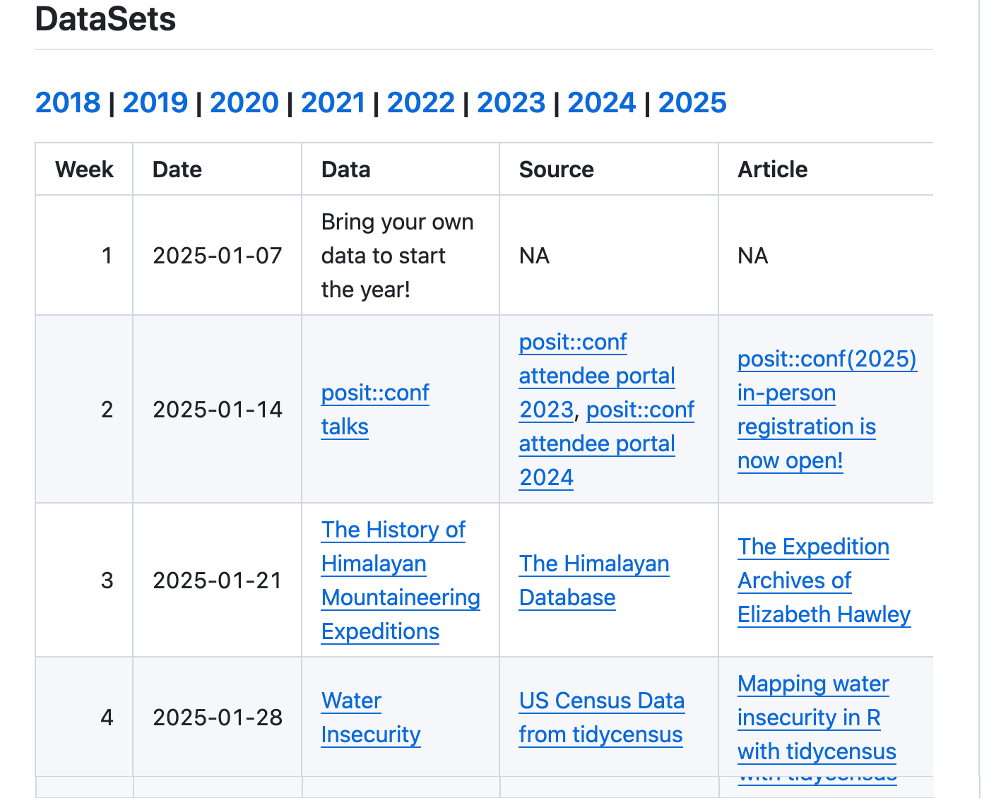
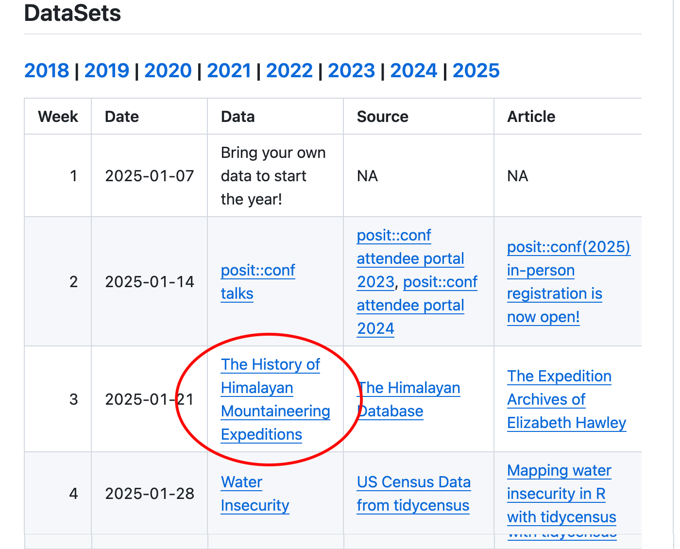
Once you find a dataset that sounds interesting, click on its link in the “Data” column.

For example, I think “The History of Himalayan Mountaineering Expeditions” dataset sounds interesting, so I’ll click on that.

“DataSets” section

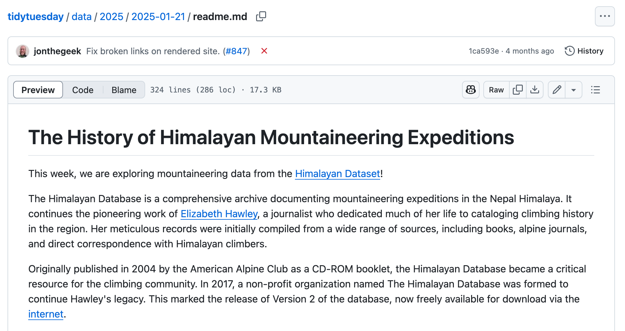
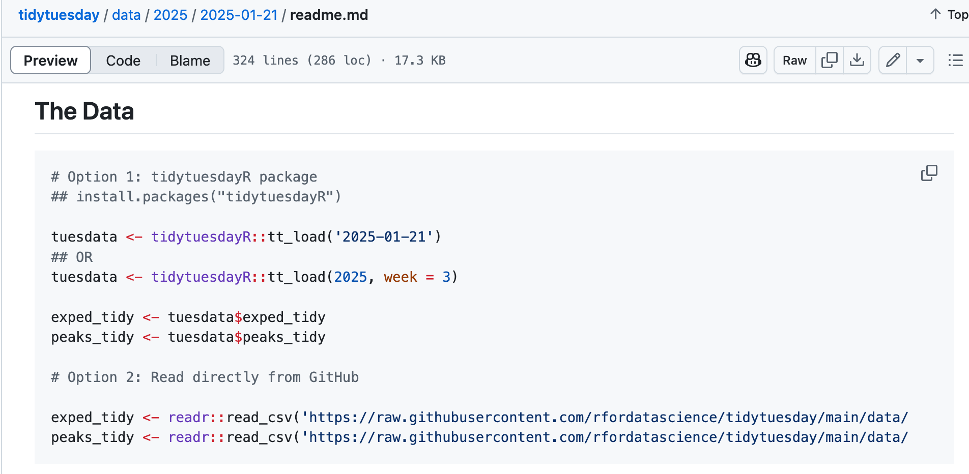
This will take us to the README file (a file that explains basic info about a piece of software, dataset, or analysis) for the “History of Himalayan Mountaineering Expeditions” dataset.

The first few paragraphs give you an overview of the dataset.

README file of the Himalayan Mountaineering Expeditions dataset

Load the data

The section called of the README file called “The Data” tells you how to load the data into R.

“The Data” section shows how to load the dataset

This is very important, because you need to load the data to analyze it.

Note that there are usually two options given for loading the data.

You only need to use one of them; option 2 is probably easier.

Option 1

The first option involves installing the “tidytuesdayR” package, which you can do with the command install.packages("tidytuesdayR").

Once you’ve installed the package, you can use it to load the data by specifying the date the data were published on TidyTuesday.

library(tidytuesdayR)

tuesdata <- tt_load("2025-01-21")
---- Compiling #TidyTuesday Information for 2025-01-21 ----
--- There are 2 files available ---


── Downloading files ───────────────────────────────────────────────────────────

  1 of 2: "exped_tidy.csv"
  2 of 2: "peaks_tidy.csv"

Note that the TidyTuesday webpage shows tidytuesdayR::tt_load("2025-01-21"), but this does the same thing as running library(tidytuesdayR) followed by tt_load("2025-01-21").

Also, when you use Option 1, the data are loaded as a list, so we need to extract each dataframe from the list. For the himalaya data, there are two dataframes. It shows us how to extract them from the list using the $ symbol:

exped_tidy <- tuesdata$exped_tidy
peaks_tidy <- tuesdata$peaks_tidy

Option 2

The second option is simpler. You can use the read_csv() function to load the data directly without installing another package.

library(tidyverse)

exped_tidy <- read_csv(
  "https://raw.githubusercontent.com/rfordatascience/tidytuesday/main/data/2025/2025-01-21/exped_tidy.csv"
)
peaks_tidy <- read_csv(
  "https://raw.githubusercontent.com/rfordatascience/tidytuesday/main/data/2025/2025-01-21/peaks_tidy.csv"
)

Take a look at the data

Now that you’ve loaded the data, have a look at it:

exped_tidy
# A tibble: 882 × 69
   EXPID     PEAKID  YEAR SEASON SEASON_FACTOR  HOST HOST_FACTOR ROUTE1   ROUTE2
   <chr>     <chr>  <dbl>  <dbl> <chr>         <dbl> <chr>       <chr>    <chr> 
 1 EVER20101 EVER    2020      1 Spring            2 China       N Col-N… <NA>  
 2 EVER20102 EVER    2020      1 Spring            2 China       N Col-N… <NA>  
 3 EVER20103 EVER    2020      1 Spring            2 China       N Col-N… <NA>  
 4 AMAD20301 AMAD    2020      3 Autumn            1 Nepal       SW Ridge <NA>  
 5 AMAD20302 AMAD    2020      3 Autumn            1 Nepal       SW Ridge <NA>  
 6 AMAD20303 AMAD    2020      3 Autumn            1 Nepal       SW Ridge <NA>  
 7 AMAD20304 AMAD    2020      3 Autumn            1 Nepal       SW Ridge <NA>  
 8 AMAD20305 AMAD    2020      3 Autumn            1 Nepal       SW Ridge <NA>  
 9 AMAD20306 AMAD    2020      3 Autumn            1 Nepal       SW Ridge <NA>  
10 AMAD20307 AMAD    2020      3 Autumn            1 Nepal       SW Ridge <NA>  
# ℹ 872 more rows
# ℹ 60 more variables: ROUTE3 <lgl>, ROUTE4 <lgl>, NATION <chr>, LEADERS <chr>,
#   SPONSOR <chr>, SUCCESS1 <lgl>, SUCCESS2 <lgl>, SUCCESS3 <lgl>,
#   SUCCESS4 <lgl>, ASCENT1 <chr>, ASCENT2 <chr>, ASCENT3 <lgl>, ASCENT4 <lgl>,
#   CLAIMED <lgl>, DISPUTED <lgl>, COUNTRIES <chr>, APPROACH <chr>,
#   BCDATE <date>, SMTDATE <date>, SMTTIME <chr>, SMTDAYS <dbl>, TOTDAYS <dbl>,
#   TERMDATE <date>, TERMREASON <dbl>, TERMREASON_FACTOR <chr>, …
peaks_tidy
# A tibble: 480 × 29
   PEAKID PKNAME      PKNAME2 LOCATION HEIGHTM HEIGHTF HIMAL HIMAL_FACTOR REGION
   <chr>  <chr>       <chr>   <chr>      <dbl>   <dbl> <dbl> <chr>         <dbl>
 1 AMAD   Ama Dablam  Amai D… Khumbu …    6814   22356    12 Khumbu            2
 2 AMPG   Amphu Gyab… Amphu … Khumbu …    5630   18471    12 Khumbu            2
 3 ANN1   Annapurna I <NA>    Annapur…    8091   26545     1 Annapurna         5
 4 ANN2   Annapurna … <NA>    Annapur…    7937   26040     1 Annapurna         5
 5 ANN3   Annapurna … <NA>    Annapur…    7555   24787     1 Annapurna         5
 6 ANN4   Annapurna … <NA>    Annapur…    7525   24688     1 Annapurna         5
 7 ANNE   Annapurna … <NA>    Annapur…    8026   26332     1 Annapurna         5
 8 ANNM   Annapurna … <NA>    Annapur…    8051   26414     1 Annapurna         5
 9 ANNS   Annapurna … Annapu… Annapur…    7219   23684     1 Annapurna         5
10 APIM   Api Main    <NA>    Api Him…    7132   23399     2 Api/Byas Ri…      7
# ℹ 470 more rows
# ℹ 20 more variables: REGION_FACTOR <chr>, OPEN <lgl>, UNLISTED <lgl>,
#   TREKKING <lgl>, TREKYEAR <dbl>, RESTRICT <chr>, PHOST <dbl>,
#   PHOST_FACTOR <chr>, PSTATUS <dbl>, PSTATUS_FACTOR <chr>, PEAKMEMO <dbl>,
#   PYEAR <dbl>, PSEASON <dbl>, PEXPID <chr>, PSMTDATE <chr>, PCOUNTRY <chr>,
#   PSUMMITERS <chr>, PSMTNOTE <chr>, REFERMEMO <dbl>, PHOTOMEMO <dbl>

Note that since there are two dataframes in this dataset, you may need to join them in order to conduct the data analysis.

Check the Data Dictionary

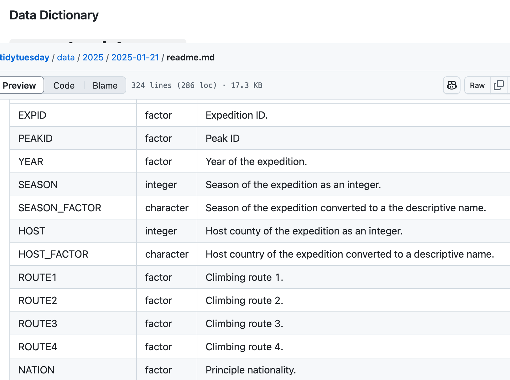
Every dataset in TidyTuesday includes a “Data Dictionary” that explains what each column in the data means. Scroll down the README file a bit further to find it. This is very important for understanding and analyzing your data.

Data Dictionary for the Himalayan Mountaineering Expeditions dataset

Start exploring the data!

For example, let’s count the names of the mountain peaks included in the peaks_tidy data:

peaks_tidy |>
  count(PKNAME)
# A tibble: 480 × 2
   PKNAME                 n
   <chr>              <int>
 1 Aichyn                 1
 2 Ama Dablam             1
 3 Amotsang               1
 4 Amphu Gyabjen          1
 5 Amphu I                1
 6 Amphu Middle           1
 7 Anidesh Chuli          1
 8 Annapurna I            1
 9 Annapurna I East       1
10 Annapurna I Middle     1
# ℹ 470 more rows

Once you get a feel for the columns in the dataset, try making some plots.

Your goal is to create a plot that tells the story hidden in the data. Good luck!